Using Tesla#
Magnetization is, according to the ontology, in Ampere per meter or equivalent.
Rather than magnetization, many people actually work with magnetic polarization in Tesla. This notebook describes how to adapt a hysteresis loop workflow in Tesla.
import math

import mammos_analysis
import mammos_dft
import mammos_entity as me
import mammos_spindynamics
import mammos_units as u
import matplotlib.pyplot as plt
import numpy as np
import pandas as pd
from mammos_mumag import hysteresis
from matplotlib import colormaps
In general, conversion between Tesla and Ampere per meter is not allowed. The following command activates the magnetic_flux_field equivalency that allows that conversion.
u.set_enabled_equivalencies(u.magnetic_flux_field())
<astropy.units.core._UnitContext at 0x7ff9ae2e4350>
Hysteresis simulation#
The function hysteresis.run requires the magnetization M to be defined in Ampere per meter, so we need to convert quantities to Tesla beforehand.
Note that although the conversion is allowed when working with Astropy Quantity, MaMMoS functions still require their inputs to be defined in SI units according to the ontology (i.e., Ampere per meter for magnetization). For example, me.M(1 * u.T) will always raise an error. So the correct strategy is to convert the Tesla value to Ampere per meter before calling the me.M() function.
(1.6 * u.T).to("A/m") # Convert 1.6 Tesla to A/m
hysteresis_result = hysteresis.run(
    mesh="cube20_singlegrain_msize2",
    Ms=me.Ms((1.6 * u.T).to("A/m")),
    A=me.A(7.7e-12, unit="J/m"),
    K1=me.Ku(4300000, unit="J/m3"),
    theta=0,
    phi=0,
    h_start=(10 * u.T).to("A/m"),
    h_final=(-10 * u.T).to("A/m"),
    h_n_steps=20,
)
Hysteresis result object and plotting#
The returned results_hysteresis contains the following values in Ampere per meter:
the external field strength
Hthe magnetization value
Mevaluated in the direction ofH.The components of the magnetization:
Mx,My,Mz.
The following cell converts the units of H and M, originally given in A/m, to Tesla (T) using the conventions \(B=\mu_0 H\) and \(J = \mu_0 M\).
B = hysteresis_result.H.q.to("T")
J = hysteresis_result.M.q.to("T")
Jx = hysteresis_result.Mx.q.to("T")
Jy = hysteresis_result.My.q.to("T")
Jz = hysteresis_result.Mz.q.to("T")
The following cell creates a dataframe df with objects in Tesla (when possible).
df = pd.DataFrame(
    {
        "configuration_type": hysteresis_result.configuration_type,
        "B": B,
        "J": J,
        "Jx": Jx,
        "Jy": Jy,
        "Jz": Jz,
        "energy_density": hysteresis_result.energy_density.q,
    }
)
df
| configuration_type | B | J | Jx | Jy | Jz | energy_density | |
|---|---|---|---|---|---|---|---|
| 0 | 1 | 10.0 | 1.599903 | -0.000029 | -0.000061 | 1.599903 | -1.672965e+07 |
| 1 | 1 | 9.0 | 1.599891 | -0.000031 | -0.000065 | 1.599891 | -1.545650e+07 |
| 2 | 1 | 8.0 | 1.599876 | -0.000033 | -0.000069 | 1.599876 | -1.418335e+07 |
| 3 | 1 | 7.0 | 1.599859 | -0.000036 | -0.000074 | 1.599859 | -1.291022e+07 |
| 4 | 1 | 6.0 | 1.599837 | -0.000038 | -0.000080 | 1.599837 | -1.163710e+07 |
| 5 | 1 | 5.0 | 1.599811 | -0.000042 | -0.000086 | 1.599811 | -1.036400e+07 |
| 6 | 1 | 4.0 | 1.599777 | -0.000046 | -0.000094 | 1.599777 | -9.090921e+06 |
| 7 | 1 | 3.0 | 1.599733 | -0.000050 | -0.000104 | 1.599733 | -7.817876e+06 |
| 8 | 1 | 2.0 | 1.599675 | -0.000056 | -0.000115 | 1.599675 | -6.544871e+06 |
| 9 | 1 | 1.0 | 1.599595 | -0.000064 | -0.000130 | 1.599595 | -5.271920e+06 |
| 10 | 1 | 0.0 | 1.599482 | -0.000073 | -0.000149 | 1.599482 | -3.999045e+06 |
| 11 | 1 | -1.0 | 1.599313 | -0.000086 | -0.000174 | 1.599313 | -2.726280e+06 |
| 12 | 1 | -2.0 | 1.599045 | -0.000105 | -0.000210 | 1.599045 | -1.453685e+06 |
| 13 | 1 | -3.0 | 1.598582 | -0.000134 | -0.000266 | 1.598582 | -1.813711e+05 |
| 14 | 1 | -4.0 | 1.597665 | -0.000186 | -0.000361 | 1.597665 | 1.090421e+06 |
| 15 | 1 | -5.0 | 1.595401 | -0.000305 | -0.000572 | 1.595401 | 2.361057e+06 |
| 16 | 1 | -6.0 | 1.585727 | -0.000966 | -0.001629 | 1.585727 | 3.627946e+06 |
| 17 | 2 | -7.0 | -1.599859 | 0.000036 | 0.000073 | -1.599859 | -1.291022e+07 |
| 18 | 2 | -8.0 | -1.599876 | 0.000033 | 0.000069 | -1.599876 | -1.418335e+07 |
| 19 | 2 | -9.0 | -1.599891 | 0.000031 | 0.000064 | -1.599891 | -1.545650e+07 |
| 20 | 2 | -10.0 | -1.599903 | 0.000029 | 0.000061 | -1.599903 | -1.672965e+07 |
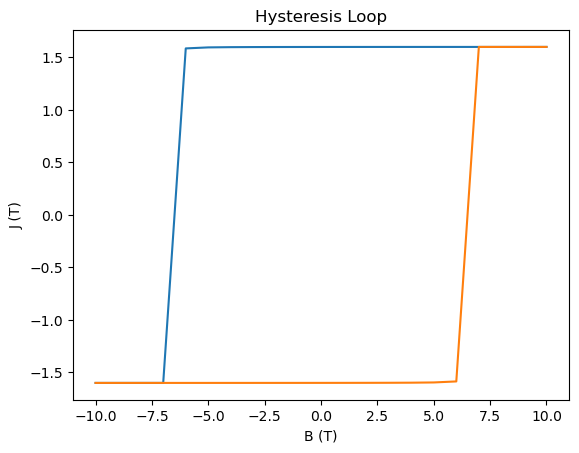
Next, we plot the hysteresis loop.
_, ax = plt.subplots()
ax.plot(B, J)
ax.plot(-B, -J)
ax.set_title("Hysteresis Loop")
ax.set_xlabel("B (T)")
ax.set_ylabel("J (T)")

plt.show();
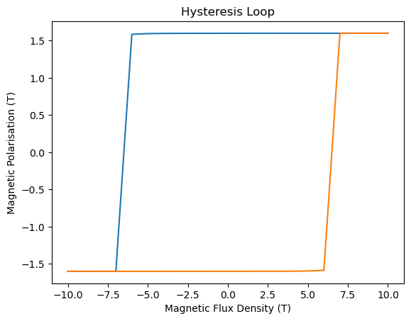
Note that it is also possible to generate a plot in Tesla using the flag Tesla=True in the plotting method of the hysteresis Result object:
hysteresis_result.plot(tesla=True);
Saving to csv file#
As the hysteresis.run function creates a hystloop.csv file in hystloop/, we want now to create another table with values converted to Tesla.
We choose the following objects from the ontology:
MagneticFluxDensity(often denoted \(\mathbf{B}\)) for the external magnetic flux densityMagneticPolarisation(\(\mathbf{J}\)) for the magnetic polarization.
me.EntityCollection(
    description="Hysteresis loop in Tesla",
    B=me.B(value=B, unit="T"),
    J=me.J(value=J, unit="T"),
    Jx=me.J(value=Jx, unit="T"),
    Jy=me.J(value=Jy, unit="T"),
    Jz=me.J(value=Jz, unit="T"),
).to_csv("hystloop_Tesla.csv")
Generate plot of \(H_c(T)\) (temperature dependent coercive field)#
In this section we show how to generate the plot from the MaMMoS Hard magnet tutorial using Celsius and Tesla
results_dft = mammos_dft.db.get_micromagnetic_properties("Fe16N2")
results_spindynamics = mammos_spindynamics.db.get_spontaneous_magnetization("Fe16N2")
results_kuzmin = mammos_analysis.kuzmin_properties(
    T=results_spindynamics.T,
    Ms=results_spindynamics.Ms,
    K1_0=results_dft.Ku_0,
)
T = np.linspace(0, 1.1 * results_kuzmin.Tc.q, 7)

simulations = []
for temperature in T:
    print(f"Running simulation for T={temperature:.0f}")
    results_hysteresis = hysteresis.run(
        mesh="cube20_singlegrain_msize2",
        Ms=results_kuzmin.Ms(temperature),
        A=results_kuzmin.A(temperature),
        K1=results_kuzmin.K1(temperature),
        theta=0,
        phi=0,
        h_start=(1.5 * u.T).to(u.A / u.m),
        h_final=(-1.5 * u.T).to(u.A / u.m),
        h_n_steps=20,
    )
    simulations.append(results_hysteresis)
Running simulation for T=0 K
Running simulation for T=215 K
Running simulation for T=430 K
Running simulation for T=644 K
Running simulation for T=859 K
Running simulation for T=1074 K
Running simulation for T=1289 K
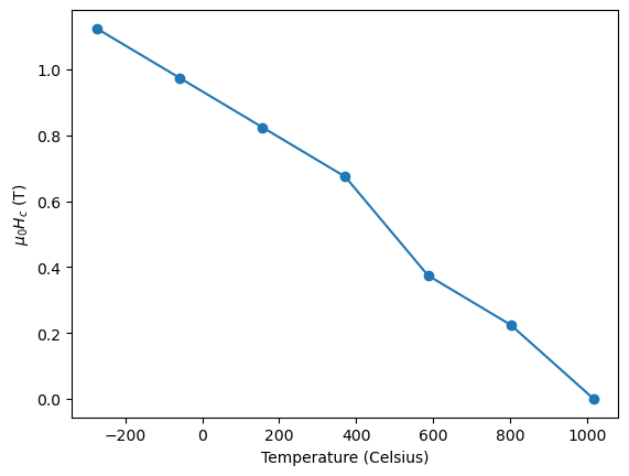
Let us visualize \(H_c(T)\), expressing the temperature Celsius and the coercive field in Tesla. For this, we need to activate the temperature equivalency on top of the previously enabled equivalencies.
u.add_enabled_equivalencies(u.temperature())
<astropy.units.core._UnitContext at 0x7ff9af250d50>
T_C = T.to("Celsius").value
Hcs_Am = []
for res in simulations:
cf = mammos_analysis.hysteresis.extract_coercive_field(H=res.H, M=res.M).q
if np.isnan(cf): # Above Tc
cf = me.Hc(0).q
Hcs_Am.append(cf) # values in A/m
Hcs_T = me.Hc(Hcs_Am).q.to("T") # values in T
plt.plot(T_C, Hcs_T, linestyle="-", marker="o")
plt.xlabel("Temperature (Celsius)")
plt.ylabel("$\mu_0 H_c$ (T)")
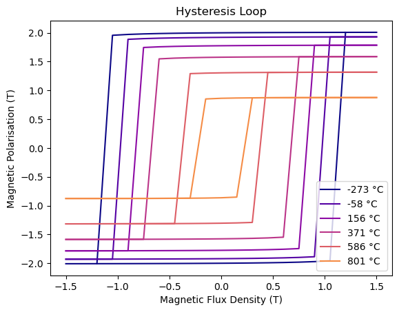
colors = colormaps["plasma"].colors[:: math.ceil(256 / len(T))]
fix, ax = plt.subplots()
for temperature, sim, color in zip(T_C, simulations, colors, strict=False):
    if np.isnan(sim.M.q).all():  # no M above Tc
        continue
    sim.plot(ax=ax, label=f"{temperature:.0f} °C", color=color, tesla=True)
ax.legend(loc="lower right");