mammos_mumag quickstart#
mammos_mumag can compute hysteresis loops of magnetic materials using finite elements.
Requirements:
mammosandesys-escript
import mammos_entity as me
import mammos_units as u
import pandas as pd
from mammos_mumag import hysteresis
u.set_enabled_equivalencies(u.magnetic_flux_field())
<astropy.units.core._UnitContext at 0x7f71dc58ccd0>
Hysteresis simulation#
The hysteresis.run function computes a hysteresis loop for a homogeneous material with given parameters. We need to pass in a suitable mesh, mammos_mumag.mesh provides a sample mesh.
hysteresis_result = hysteresis.run(
    mesh="cube20_singlegrain_msize2",
    Ms=me.Ms(1280000, unit="A/m"),
    A=me.A(7.7e-12, unit="J/m"),
    K1=me.Ku(4300000, unit="J/m3"),
    theta=0,
    phi=0,
    h_start=(10 * u.T).to("A/m"),
    h_final=(-10 * u.T).to("A/m"),
    h_n_steps=20,
)
Hysteresis result object#
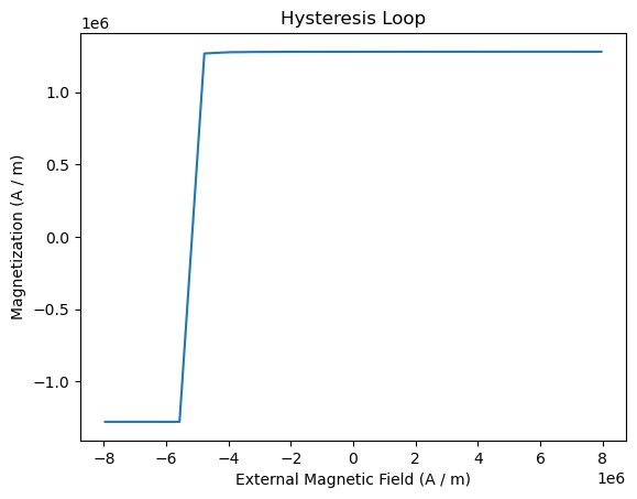
The returned results_hysteresis object provides a plot method to visualize the computed data. mammos_mumag.hysteresis only computes half a hysteresis loop, going from hstart to hfinal. To show a full loop this function mirrors the computed data and plots it twice:
hysteresis_result.plot();

To only see the actual simulation, we can use the flag duplicate=False:
hysteresis_result.plot(duplicate=False);
The results object provides access to:
the external field
Hthe magnetization
Min the direction of the applied fieldthe components
Mx,My,Mzof the magnetizationthe energy density
hysteresis_result.H
[ 7957747.15026276 7161972.43523649 6366197.72021021 5570423.00518393
4774648.29015766 3978873.57513138 3183098.86010511 2387324.14507883
1591549.43005255 795774.71502628 0. -795774.71502628
-1591549.43005255 -2387324.14507883 -3183098.86010511 -3978873.57513138
-4774648.29015766 -5570423.00518393 -6366197.72021021 -7161972.43523649
-7957747.15026276],
unit=A / m)
hysteresis_result.M
[ 1279920.92569655 1279911.14633934 1279899.42963877 1279885.2268147
1279867.77972873 1279846.01687668 1279818.38389404 1279782.55594664
1279734.92828792 1279669.66402409 1279576.79658277 1279438.13222608
1279217.45234696 1278833.60909754 1278070.51029595 1276161.36652649
1267635.43145344 -1279885.22584968 -1279899.42846665 -1279911.1452972
-1279920.92579483],
unit=A / m)
hysteresis_result.Mx
[ -23.54037126 -25.0451965 -26.7560345 -28.71848504 -30.99269791
-33.65924931 -36.82966917 -40.66202659 -45.38837715 -51.36375841
-59.15966038 -69.76275253 -85.0222662 -108.88273736 -151.57027633
-250.75175893 -861.56501265 28.53876135 26.72983079 25.0250458
23.51679169],
unit=A / m)
hysteresis_result.My
[ -48.9635178 -52.0457853 -55.54281008 -59.54464247
-64.16984798 -69.57549466 -75.97863179 -83.68435754
-93.13691972 -105.00949446 -120.37511784 -141.05920632
-170.42606819 -215.51717585 -294.12895559 -469.64559154
-1433.18253466 59.01421681 55.28635356 51.8495188
48.99411012],
unit=A / m)
hysteresis_result.Mz
[ 1279920.92569655 1279911.14633934 1279899.42963877 1279885.2268147
1279867.77972873 1279846.01687668 1279818.38389404 1279782.55594664
1279734.92828792 1279669.66402409 1279576.79658277 1279438.13222608
1279217.45234696 1278833.60909754 1278070.51029595 1276161.36652649
1267635.43145344 -1279885.22584968 -1279899.42846665 -1279911.1452972
-1279920.92579483],
unit=A / m)
hysteresis_result.energy_density
[-16794046.39939273 -15514130.21974726 -14234224.74917092
-12954332.18513003 -11674455.37178373 -10394598.05726379
-9114765.28465126 -7834964.0056009 -6555204.08037736
-5275499.98242484 -3995873.86585082 -2716361.46928677
-1437024.49582884 -157979.70553049 1120520.7665673
2397803.50265979 3671036.31564498 -12954332.18511862
-14234224.74916488 -15514130.2197436 -16794046.39939053],
unit=J / m3)
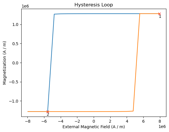
The attribute configuration_type contains a list of indices that refer to saved magnetization field configurations. We will use this information later.
hysteresis_result.configuration_type
array([1, 1, 1, 1, 1, 1, 1, 1, 1, 1, 1, 1, 1, 1, 1, 1, 1, 2, 2, 2, 2])
We can also get the hysteresis data as a pandas dataframe in SI units:
hysteresis_result.dataframe
| configuration_type | H | M | Mx | My | Mz | energy_density | |
|---|---|---|---|---|---|---|---|
| 0 | 1 | 7.957747e+06 | 1.279921e+06 | -23.540371 | -48.963518 | 1.279921e+06 | -1.679405e+07 |
| 1 | 1 | 7.161972e+06 | 1.279911e+06 | -25.045197 | -52.045785 | 1.279911e+06 | -1.551413e+07 |
| 2 | 1 | 6.366198e+06 | 1.279899e+06 | -26.756035 | -55.542810 | 1.279899e+06 | -1.423422e+07 |
| 3 | 1 | 5.570423e+06 | 1.279885e+06 | -28.718485 | -59.544642 | 1.279885e+06 | -1.295433e+07 |
| 4 | 1 | 4.774648e+06 | 1.279868e+06 | -30.992698 | -64.169848 | 1.279868e+06 | -1.167446e+07 |
| 5 | 1 | 3.978874e+06 | 1.279846e+06 | -33.659249 | -69.575495 | 1.279846e+06 | -1.039460e+07 |
| 6 | 1 | 3.183099e+06 | 1.279818e+06 | -36.829669 | -75.978632 | 1.279818e+06 | -9.114765e+06 |
| 7 | 1 | 2.387324e+06 | 1.279783e+06 | -40.662027 | -83.684358 | 1.279783e+06 | -7.834964e+06 |
| 8 | 1 | 1.591549e+06 | 1.279735e+06 | -45.388377 | -93.136920 | 1.279735e+06 | -6.555204e+06 |
| 9 | 1 | 7.957747e+05 | 1.279670e+06 | -51.363758 | -105.009494 | 1.279670e+06 | -5.275500e+06 |
| 10 | 1 | 0.000000e+00 | 1.279577e+06 | -59.159660 | -120.375118 | 1.279577e+06 | -3.995874e+06 |
| 11 | 1 | -7.957747e+05 | 1.279438e+06 | -69.762753 | -141.059206 | 1.279438e+06 | -2.716361e+06 |
| 12 | 1 | -1.591549e+06 | 1.279217e+06 | -85.022266 | -170.426068 | 1.279217e+06 | -1.437024e+06 |
| 13 | 1 | -2.387324e+06 | 1.278834e+06 | -108.882737 | -215.517176 | 1.278834e+06 | -1.579797e+05 |
| 14 | 1 | -3.183099e+06 | 1.278071e+06 | -151.570276 | -294.128956 | 1.278071e+06 | 1.120521e+06 |
| 15 | 1 | -3.978874e+06 | 1.276161e+06 | -250.751759 | -469.645592 | 1.276161e+06 | 2.397804e+06 |
| 16 | 1 | -4.774648e+06 | 1.267635e+06 | -861.565013 | -1433.182535 | 1.267635e+06 | 3.671036e+06 |
| 17 | 2 | -5.570423e+06 | -1.279885e+06 | 28.538761 | 59.014217 | -1.279885e+06 | -1.295433e+07 |
| 18 | 2 | -6.366198e+06 | -1.279899e+06 | 26.729831 | 55.286354 | -1.279899e+06 | -1.423422e+07 |
| 19 | 2 | -7.161972e+06 | -1.279911e+06 | 25.025046 | 51.849519 | -1.279911e+06 | -1.551413e+07 |
| 20 | 2 | -7.957747e+06 | -1.279921e+06 | 23.516792 | 48.994110 | -1.279921e+06 | -1.679405e+07 |
We can generate a table in alternate units:
df = pd.DataFrame(
    {
        "mu0_H": hysteresis_result.H.q.to(u.T),
        "J": hysteresis_result.M.q.to(u.T),
    },
)
df.head()
| mu0_H | J | |
|---|---|---|
| 0 | 10.0 | 1.608396 |
| 1 | 9.0 | 1.608384 |
| 2 | 8.0 | 1.608369 |
| 3 | 7.0 | 1.608351 |
| 4 | 6.0 | 1.608329 |
Visualizing magnetization configurations#
To plot the hysteresis loop (including the available configurations), run
hysteresis_result.plot(configuration_marks=True);
We can get the location of the saved configurations from the attribute configurations:
hysteresis_result.configurations
{1: PosixPath('/tmp/tmpyuytlj_t/hystloop/hystloop_0001.vtu'),
 2: PosixPath('/tmp/tmpyuytlj_t/hystloop/hystloop_0002.vtu')}
To inspect the configurations more conveniently directly in the notebook we can use the plot_configuration function of hysteresis_result. We need to pass the index and get an interactive 3D plot (using pyvista):
hysteresis_result.plot_configuration(1)
/home/runner/work/mammos/mammos/.pixi/envs/docs/lib/python3.11/site-packages/pyvista/jupyter/notebook.py:37: UserWarning: Failed to use notebook backend:

Please install `nest_asyncio` to automagically launch the trame server without await. Or, to avoid `nest_asynctio` run:

    from pyvista.trame.jupyter import launch_server
    await launch_server().ready


Falling back to a static output.
  warnings.warn(
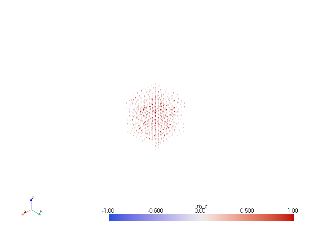
Note: the small object size is a consequence of the empty sphere around the cube.