Hysteresis loop simulation#
The notebook shows how to run micromagnetic simulations to obtain a hysteresis loop for a magnetic material. The workflow involves defining a:
geometry and mesh which discretizes the material into cells for numerical calculations, and also defines sub-regions within the material.
micromagnetic material parameters corresponding to different sub-regions.
simulation parameters which control the simulation algorithms.
All of the above mentioned definitions are used to create a simulation object which will be used to actually run the hysteresis loop simulation. The simulation run will store magnetization configuration in vtu file(s). Further, it will create a csv file that contains magnitude of external field, magnetization in the direction of the external field, components of average magnetization, and total energy. Finally, the simulation run stores the time and version of mammos_mumag in an info.json file.
import mammos_entity as me
import mammos_units as u
from mammos_mumag.hysteresis import read_result
from mammos_mumag.materials import Materials
from mammos_mumag.mesh import Mesh
from mammos_mumag.parameters import Parameters
from mammos_mumag.simulation import Simulation

u.set_enabled_equivalencies(u.magnetic_flux_field());
Inputs#
Geometry and Mesh#
We load one of the meshes coming with mammos_mumag, cube20_singlegrain_msize2, defining a cube of length 20 with no grains and a mesh size of 2. The cube is surrounded by a shell and non-magnetic material in between the material cube and the shell. This is done is order to calculate demagnetization field which decays to zero at infinity. For details: Imhoff, J. F., et al. “An original solution for unbounded electromagnetic 2D-and 3D-problems throughout the finite element method.” IEEE Transactions on Magnetics 26.5 (1990): 1659-1661.
mesh = Mesh("cube20_singlegrain_msize2")
Material parameters#
We define the material parameters separately for the 3 domains: the magnetic material, the non-magnetic material and the shell. Therefore the parameters strictly related to the magnetic material will be only defined on the first domain. The other domains will have magnetic properties equal to zero.
Here:
thetais the polar angle of the magneto-crystalline anisotropy with respect to z-axis.phiis the azimuthal angle of the magneto-crystalline anisotropy in the xy-plane with respect to x-axis.K1is the first order magneto-crystalline anisotropy constant.Msis the spontaneous magnetization.Ais the exchange stiffness constant.
mat = Materials(
    domains=[
        {  # cube
            "theta": 0.0,
            "phi": 0.0,
            "K1": me.Ku(2.8e6, unit=u.J / u.m**3),
            "Ms": me.Ms(1.19e6, unit=u.A / u.m),
            "A": me.A(6.01e-12, unit=u.J / u.m),
        },
        {  # non-magnetic material
            "theta": 0.0,
            "phi": 0.0,
            "K1": me.Ku(0.0, unit=u.J / u.m**3),
            "Ms": me.Ms(0.0, unit=u.A / u.m),
            "A": me.A(0.0, unit=u.J / u.m),
        },
        {  # shell
            "theta": 0.0,
            "phi": 0.0,
            "K1": me.Ku(0.0, unit=u.J / u.m**3),
            "Ms": me.Ms(0.0, unit=u.A / u.m),
            "A": me.A(0.0, unit=u.J / u.m),
        },
    ],
)
Simulation parameters#
We finally define all the simulation parameters we will use. For an exhaustive explanation of these parameters, check the documentation.
par = Parameters(
    size=1.0e-9,
    scale=0,
    m_vect=[0, 0, 1],
    h_start=(10 * u.T).to("A/m"),
    h_final=(-10 * u.T).to("A/m"),
    h_step=(-2 * u.T).to("A/m"),
    h_vect=[0.01745, 0, 0.99984],
    m_step=(0.4 * u.T).to("A/m"),
    m_final=(-1.2 * u.T).to("A/m"),
    tol_fun=1e-10,
    tol_h_mag_factor=1,
    precond_iter=10,
)
Simulation object#
To define a Simulation object, we need to define a mesh, a Materials object, and a Parameters object as shown above.
sim = Simulation(
    mesh=mesh,
    materials=mat,
    parameters=par,
)
Note that all of this could also have been defined using file paths:
sim = Simulation(
    mesh=Mesh("./mesh.fly"),
    materials_filepath="./material.krn",
    parameters_filepath="./sim-settings.p2",
)
Hysteresis loop calculation#
To compute the demagnetization curve, we use sim.run_loop method. Here, we can specify the optional argument outdir and name. While the first identifies the output directory where the input and output files will be stored (also where the script is executed), the name argument defines the names of the output files.
The outdir argument can be used to give an ID to the simulation.
sim.run_loop(outdir="out/loop", name="cube")
The out/loop directory looks like:
$> tree out/loop/
out/loop
├── cube_0001.vtu
├── cube_0002.vtu
├── cube.csv
├── cube.fly
├── cube.krn
├── cube.p2
├── cube_stats.txt
└── info.json
Simulation results#
The simulation results can be loaded into a mammos_mumag.hysteresis.Result object using mammos_mumag.hysteresis.read_result function.
results = read_result(outdir="out/loop", name="cube")
results
Result(H=Entity(ontology_label='ExternalMagneticField', value=array([ 7957747.15026276,  6366197.72021021,  4774648.29015766,
        3183098.86010511,  1591549.43005255,        0.        ,
       -1591549.43005255, -3183098.86010511, -4774648.29015766]), unit='A / m'), M=Entity(ontology_label='Magnetization', value=array([ 1189898.9481906 ,  1189866.40526925,  1189815.11921464,
        1189727.28638435,  1189557.43497599,  1189157.86904957,
        1187783.07668437,  1164137.60418793, -1189815.1228945 ]), unit='A / m'), Mx=Entity(ontology_label='Magnetization', value=array([ 1.40977658e+04,  1.30478457e+04,  1.16056500e+04,  9.50089294e+03,
        6.14117264e+03, -7.34109511e+01, -1.54960020e+04, -1.47662455e+05,
       -1.16058801e+04]), unit='A / m'), My=Entity(ontology_label='Magnetization', value=array([  -47.99514144,   -55.4713862 ,   -65.7111453 ,   -80.59786012,
        -104.24878947,  -147.68486853,  -254.6017913 , -1655.25070268,
          65.72948994]), unit='A / m'), Mz=Entity(ontology_label='Magnetization', value=array([ 1189834.11060143,  1189819.88676161,  1189793.76323892,
        1189742.65092037,  1189631.41014654,  1189340.24520851,
        1188234.41075948,  1166892.01100325, -1189793.7629022 ]), unit='A / m'), energy_density=Entity(ontology_label='EnergyDensity', value=array([-14435045.7150797 , -12055278.0880263 ,  -9675592.39554646,
        -7296041.45406551,  -4916736.1890445 ,  -2537956.76779954,
         -160685.1661964 ,   2205885.87471876,  -9675592.39554454]), unit='J / m3'), configuration_type=array([1, 1, 1, 1, 1, 1, 1, 1, 2]), configurations={1: PosixPath('/tmp/tmp596kct54/out/loop/cube_0001.vtu'), 2: PosixPath('/tmp/tmp596kct54/out/loop/cube_0002.vtu')})
The Result object stores the magnitude of external magnetic field along a direction defined using h_vect in Parameters object, the magnitude of magnetization along the same direction, and total energy density of the system as mammos_entity.Entity objects.
results.H
[ 7957747.15026276 6366197.72021021 4774648.29015766 3183098.86010511
1591549.43005255 0. -1591549.43005255 -3183098.86010511
-4774648.29015766],
unit=A / m)
results.M
[ 1189898.9481906 1189866.40526925 1189815.11921464 1189727.28638435
1189557.43497599 1189157.86904957 1187783.07668437 1164137.60418793
-1189815.1228945 ],
unit=A / m)
results.energy_density
[-14435045.7150797 -12055278.0880263 -9675592.39554646
-7296041.45406551 -4916736.1890445 -2537956.76779954
-160685.1661964 2205885.87471876 -9675592.39554454],
unit=J / m3)
It is also possible to convert the data points of the outputs into a pandas.DataFrame.
results.dataframe
| configuration_type | H | M | Mx | My | Mz | energy_density | |
|---|---|---|---|---|---|---|---|
| 0 | 1 | 7.957747e+06 | 1.189899e+06 | 14097.765759 | -47.995141 | 1.189834e+06 | -1.443505e+07 |
| 1 | 1 | 6.366198e+06 | 1.189866e+06 | 13047.845667 | -55.471386 | 1.189820e+06 | -1.205528e+07 |
| 2 | 1 | 4.774648e+06 | 1.189815e+06 | 11605.649969 | -65.711145 | 1.189794e+06 | -9.675592e+06 |
| 3 | 1 | 3.183099e+06 | 1.189727e+06 | 9500.892936 | -80.597860 | 1.189743e+06 | -7.296041e+06 |
| 4 | 1 | 1.591549e+06 | 1.189557e+06 | 6141.172644 | -104.248789 | 1.189631e+06 | -4.916736e+06 |
| 5 | 1 | 0.000000e+00 | 1.189158e+06 | -73.410951 | -147.684869 | 1.189340e+06 | -2.537957e+06 |
| 6 | 1 | -1.591549e+06 | 1.187783e+06 | -15496.002030 | -254.601791 | 1.188234e+06 | -1.606852e+05 |
| 7 | 1 | -3.183099e+06 | 1.164138e+06 | -147662.454940 | -1655.250703 | 1.166892e+06 | 2.205886e+06 |
| 8 | 2 | -4.774648e+06 | -1.189815e+06 | -11605.880141 | 65.729490 | -1.189794e+06 | -9.675592e+06 |
configuration_type: the id of the magnetization vector field appended to thevtufile name. Thevtufiles contain the magnetization corresponding to the row where the given value ofidxwas first observed.H: the value of the external field (\(H_{\mathsf{ext}}\)) in A/m.M: the magnitude of average magnetization (\(M\)), in A/m, parallel to the direction of the external field.Mx: the component of average magnetization in x direction in A/m.My: the component of average magnetization in y direction in A/m.Mz: the component of average magnetization in z direction in A/m.energy_density: the energy density (in J/m\(^3\)) of the current state.
To plot the hysteresis curve, use plot method of the Result object.
results.plot();
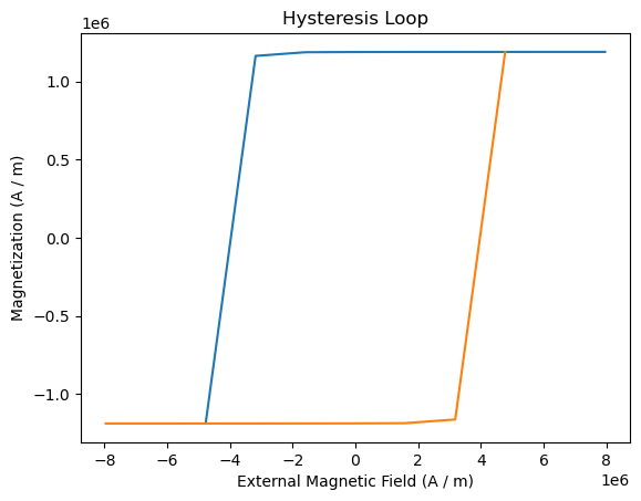
NOTE: the orange curve in the plot above is artificially added to complete a full hysteresis loop. whether to show it or not can be controlled by the
duplicateparameter of theplotmethod.
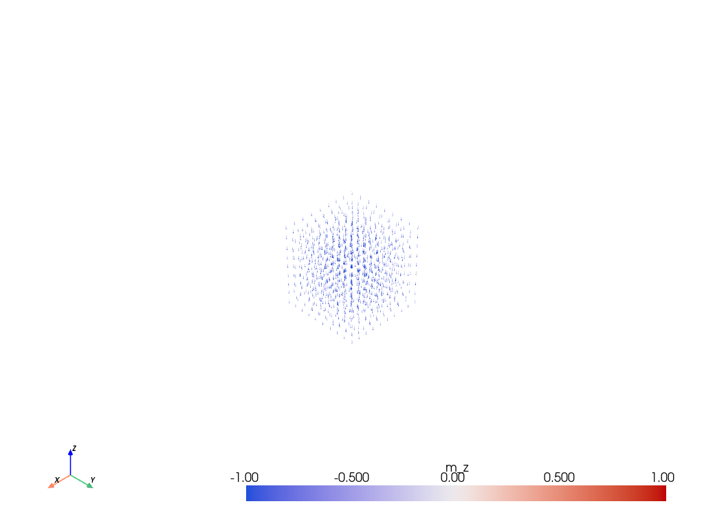
The Result object also contains the magnetization configurations corresponding to the different configuration_types.
results.configurations
{1: PosixPath('/tmp/tmp596kct54/out/loop/cube_0001.vtu'),
 2: PosixPath('/tmp/tmp596kct54/out/loop/cube_0002.vtu')}
To plot the configurations, use plot_configuration method of the Result object.
results.plot_configuration(2)
/home/runner/work/mammos/mammos/.pixi/envs/docs/lib/python3.11/site-packages/pyvista/jupyter/notebook.py:37: UserWarning: Failed to use notebook backend:

Please install `nest_asyncio` to automagically launch the trame server without await. Or, to avoid `nest_asynctio` run:

    from pyvista.trame.jupyter import launch_server
    await launch_server().ready


Falling back to a static output.
  warnings.warn(
NOTE: It is important to note that there is a convenience function mammos_mumag.hysteresis.run that does not require the user to input detailed material and simulation parameters to run hysteresis simulations.