Sensor shape optimization workflow#

In this example we will show how to use MaMMoS for shape optimization of a magnetic sensor element. To show the versatility of the mammos software we will perform the micromagnetic simulations with the ubermag micromagnetic package.

In this workflow we optimize the region of the hysteresis loop over which M vs H has a linear reponse. In order to do this we will first obtain micromagnetic parameters, perform micromagnetic simulations, and then analyze the hysteresis loop.

This is followed by Baysian optimization to maximize the linear region.

Requirements:

Software: mammos, ubermag with OOMMF, bayesian-optimization
Basic understanding of mammos-units and mammos-entity

[1]:

%config InlineBackend.figure_format = "retina"

# MaMMoS imports
# Ubermag imports
import discretisedfield as df
import mammos_analysis
import mammos_entity as me
import mammos_spindynamics
import mammos_units as u
import micromagneticdata as md
import micromagneticmodel as mm
import numpy as np
import oommfc as mc

[2]:

%config InlineBackend.figure_format = "retina"

[3]:

# Allow convenient conversions between A/m and T
u.set_enabled_equivalencies(u.magnetic_flux_field());

Temperature-dependent magnetization data from spindynamics database lookup#

In order to get micromagnetic parameters we use pre-computed data from mammos_spindynamics.db for the temperature-dependent magnetization.

[4]:

results_spindynamics = mammos_spindynamics.db.get_spontaneous_magnetization("Ni80Fe20")

We can visualize the pre-computed data using .plot.

[5]:

results_spindynamics.plot(marker="X");

../../_images/examples_workflows_sensor_7_0.png

We can access T and Ms and get mammos_entity.Entity objects:

[6]:

results_spindynamics.T

[6]:

ThermodynamicTemperature(value=
[   0.   10.   20.   30.   40.   50.   60.   70.   80.   90.  100.  110.
  120.  130.  140.  150.  160.  170.  180.  190.  200.  210.  220.  230.
  240.  250.  260.  270.  280.  290.  300.  310.  320.  330.  340.  350.
  360.  370.  380.  390.  400.  410.  420.  430.  440.  450.  460.  470.
  480.  490.  500.  510.  520.  530.  540.  550.  560.  570.  580.  590.
  600.  610.  620.  630.  640.  650.  660.  670.  680.  690.  700.  710.
  720.  730.  740.  750.  760.  770.  780.  790.  800.  810.  820.  830.
  840.  850.  860.  870.  880.  890.  900.  910.  920.  930.  940.  950.
  960.  970.  980.  990. 1000.],
 unit=K)

[7]:

results_spindynamics.Ms

[7]:

SpontaneousMagnetization(value=
[892184.69121101 891969.67470043 891513.76832322 890894.59214752
 890083.59626321 889199.44123422 888171.64446995 887053.73705186
 885671.74296517 884395.91885674 883079.94643721 881495.42642562
 879788.67711133 877788.39903363 875834.51455988 874081.37164165
 872049.86709976 869912.19257962 867442.62535435 865562.79220997
 863209.20899455 860457.71140686 857763.3136394  855296.4229682
 852466.41312768 849523.98801607 846414.7243672  842904.86979197
 840148.91128082 836734.52046756 833918.7855821  830963.86988481
 827691.33643744 824071.7431452  819584.05414841 816187.50702897
 812565.23718265 809168.69006321 805466.12359469 800465.42840045
 796733.41983711 791036.82058373 787268.23244806 784894.12898474
 777771.81859481 774073.71304974 767972.95413124 764328.37966764
 758786.12836584 752673.77104635 746867.43307595 739287.43193942
 734194.84172199 730168.41221055 722195.84980989 716598.28305723
 712643.22832109 704576.09434316 696401.89820229 692470.93245281
 680049.93718177 676438.37355175 666863.44744567 656975.36451298
 651927.38353011 640064.00369108 630156.29269518 624160.81157024
 609419.24391736 603364.8786028  595334.32419721 584191.82958868
 572021.53821587 561564.24145018 543284.26931196 533357.82243755
 514577.33468756 508894.11820454 485029.96208403 462149.88567792
 445504.395894   414821.27217856 393520.3626759  363208.387792
 334083.91073211 292258.29240814 222773.16428724 150432.15296978
  36090.5659104   32874.68619093  19763.85371664  32641.20145724
   6222.41722299  14944.80732554  18460.81797513  12186.88600807
  10183.9313763    6629.18206741  13175.69430134   9669.14080947
   6273.31635963],
 unit=A / m)

Calculate micromagnetic intrinsic properties using Kuz’min formula#

We use Kuz’min equations to compute Ms(T) and A(T).

[8]:

kuzmin_result = mammos_analysis.kuzmin_properties(
    T=results_spindynamics.T,
    Ms=results_spindynamics.Ms,
)

[9]:

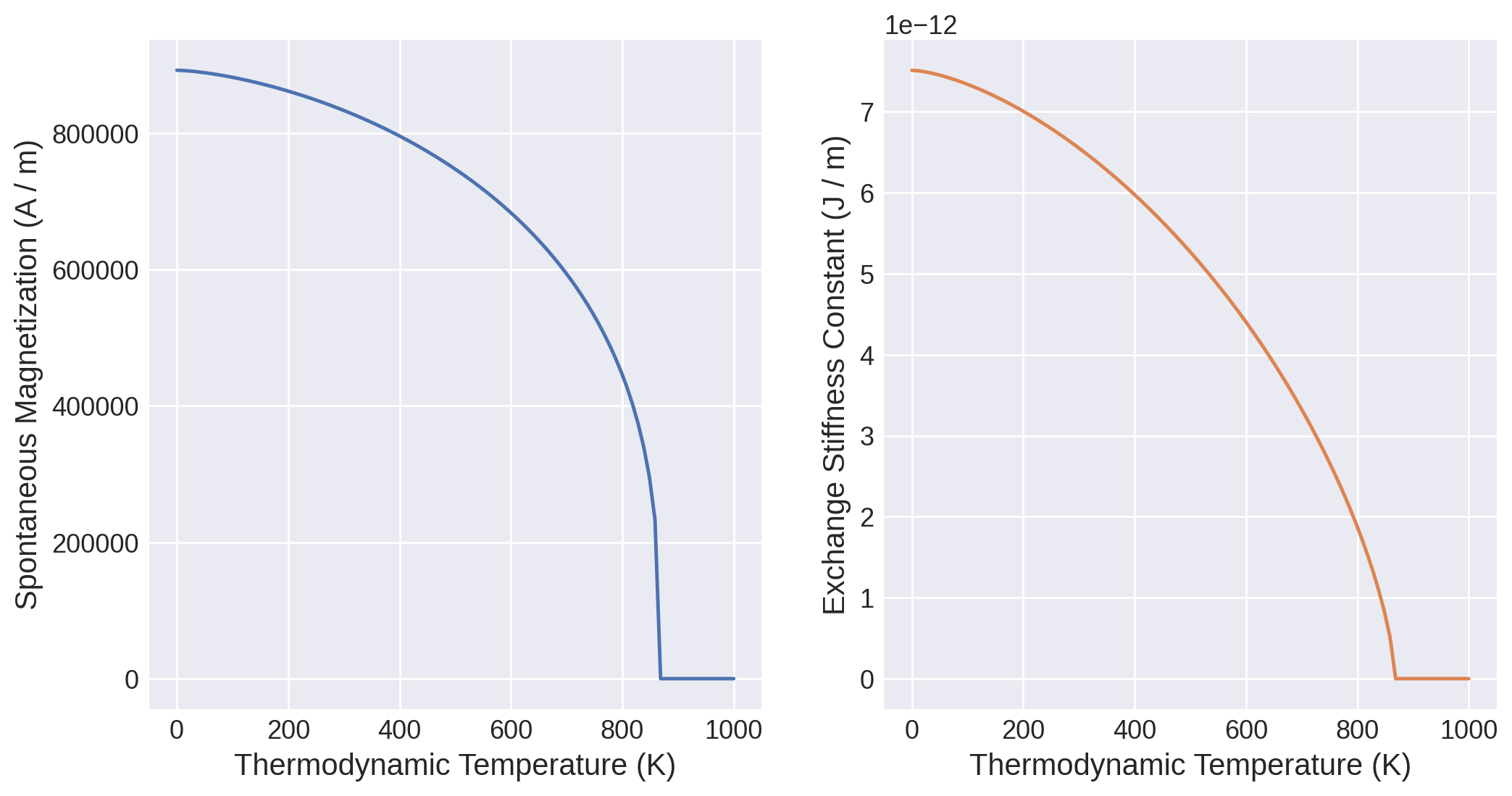
kuzmin_result.plot();

../../_images/examples_workflows_sensor_13_0.png

[10]:

kuzmin_result

[10]:

KuzminResult(Ms=Ms(T), A=A(T), Tc=CurieTemperature(value=868.103292637747, unit=K), s=<Quantity 0.86884674>, K1=None)

[11]:

kuzmin_result.Ms(0)

[11]:

SpontaneousMagnetization(value=892184.691211015, unit=A / m)

[12]:

kuzmin_result

[12]:

KuzminResult(Ms=Ms(T), A=A(T), Tc=CurieTemperature(value=868.103292637747, unit=K), s=<Quantity 0.86884674>, K1=None)

[13]:

kuzmin_result.Ms(0)

[13]:

SpontaneousMagnetization(value=892184.691211015, unit=A / m)

Setting up the micromagnetic simulation#

Run the micromagnetic simulation with parameters at 300 K using ubermag with OOMMF as calculator.

[14]:

T = me.T(300, unit="K")

Define the energy equation of the system.

[15]:

system = mm.System(name="sensor")
A = kuzmin_result.A(T)
Ms = kuzmin_result.Ms(T)
system.energy = mm.Exchange(A=A.value) + mm.Demag() + mm.Zeeman(H=(0, 0, 0))

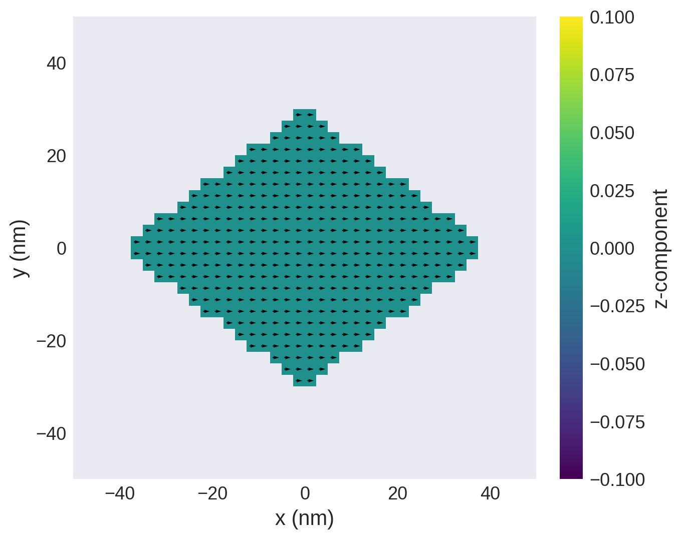
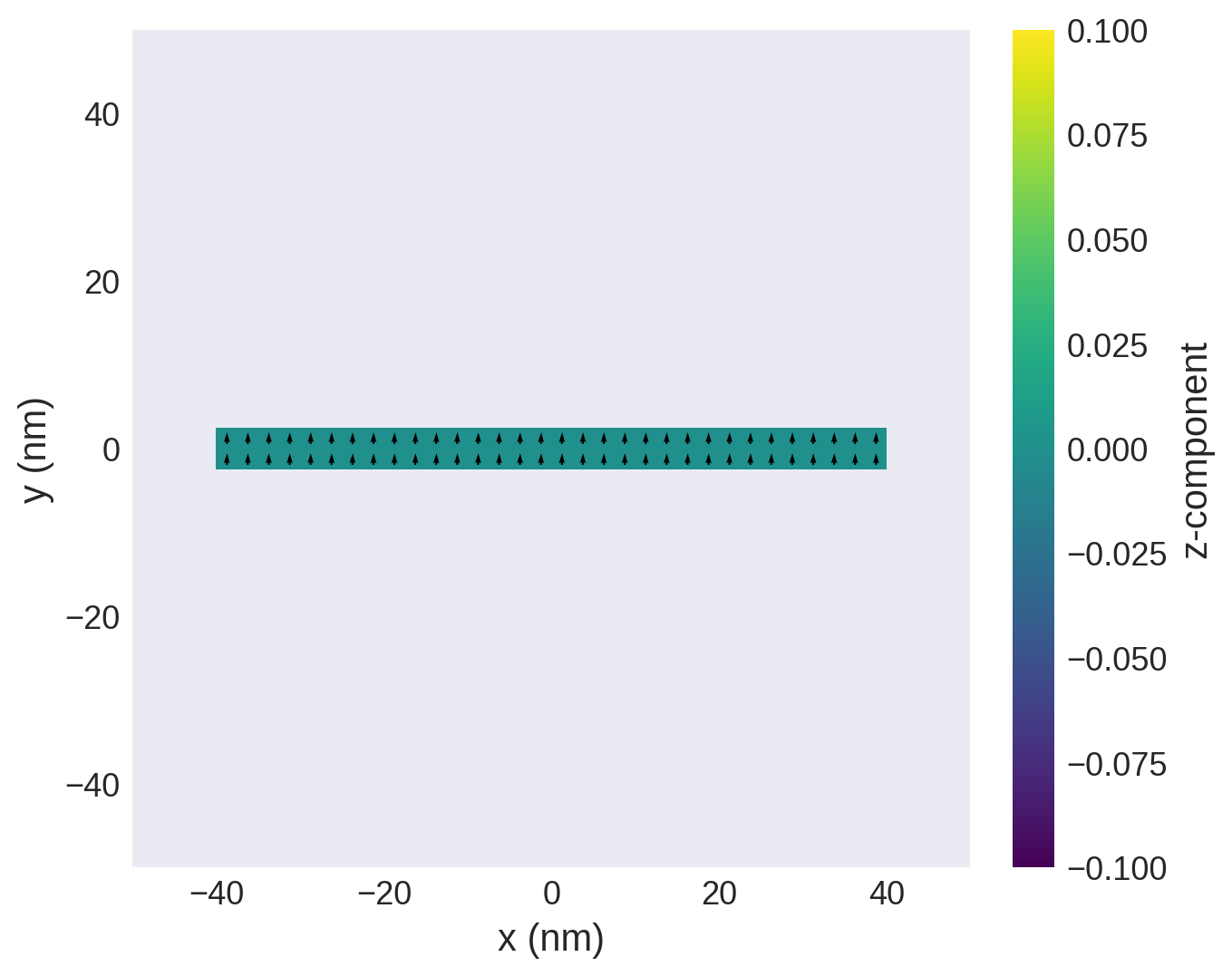
Initialize the magnetization: we constrain the shape of our sensor to be a diamond (rhombus) with the distance $s_x$ and $s_y$ from origin to corners along the $x$ and $y$ directions, respectively, and with thickness $t$. We create a $100\times 100\times 5$ nm region in which we create the diamond shape of magnetic material.

[16]:

L = 100e-9  # nm
t = 5e-9  # nm
region = df.Region(p1=(-L / 2, -L / 2, -t / 2), p2=(L / 2, L / 2, t / 2))
mesh = df.Mesh(region=region, n=(40, 40, 1))


def in_diamond(position, sx, sy):
    x, y, _ = position
    if abs(x) / sx + abs(y) / sy <= 1:
        return Ms.value
    else:
        return 0


system.m = df.Field(mesh, nvdim=3, value=(1, 0, 0), norm=lambda p: in_diamond(p, 40e-9, 30e-9), valid="norm")

[17]:

system.m.sel("z").mpl()

../../_images/examples_workflows_sensor_24_0.png

Run a hystersis loop from 0 to 500 mT in the y direction:

[18]:

Hmin = (0, 0, 0)
Hmax = ((0.1, 500, 0) * u.mT).to(u.A / u.m)  # Convert to A/m for Ubermag compatibility
n = 101

hd = mc.HysteresisDriver()
hd.drive(system, Hsteps=[[Hmin, tuple(Hmax.value), n]])

Running OOMMF (ExeOOMMFRunner)[2025-06-06T16:56:38]... (5.3 s)

Extract entitles from the results of our field sweep:

[19]:

H_y = me.H(
    system.table.data["By_hysteresis"].values  # simulation output in mT
    * u.Unit(system.table.units["By_hysteresis"]).to(u.A / u.m)  # conversion factor from mT to A/m
)
M_y = me.Entity("Magnetization", system.table.data["my"].values * Ms)

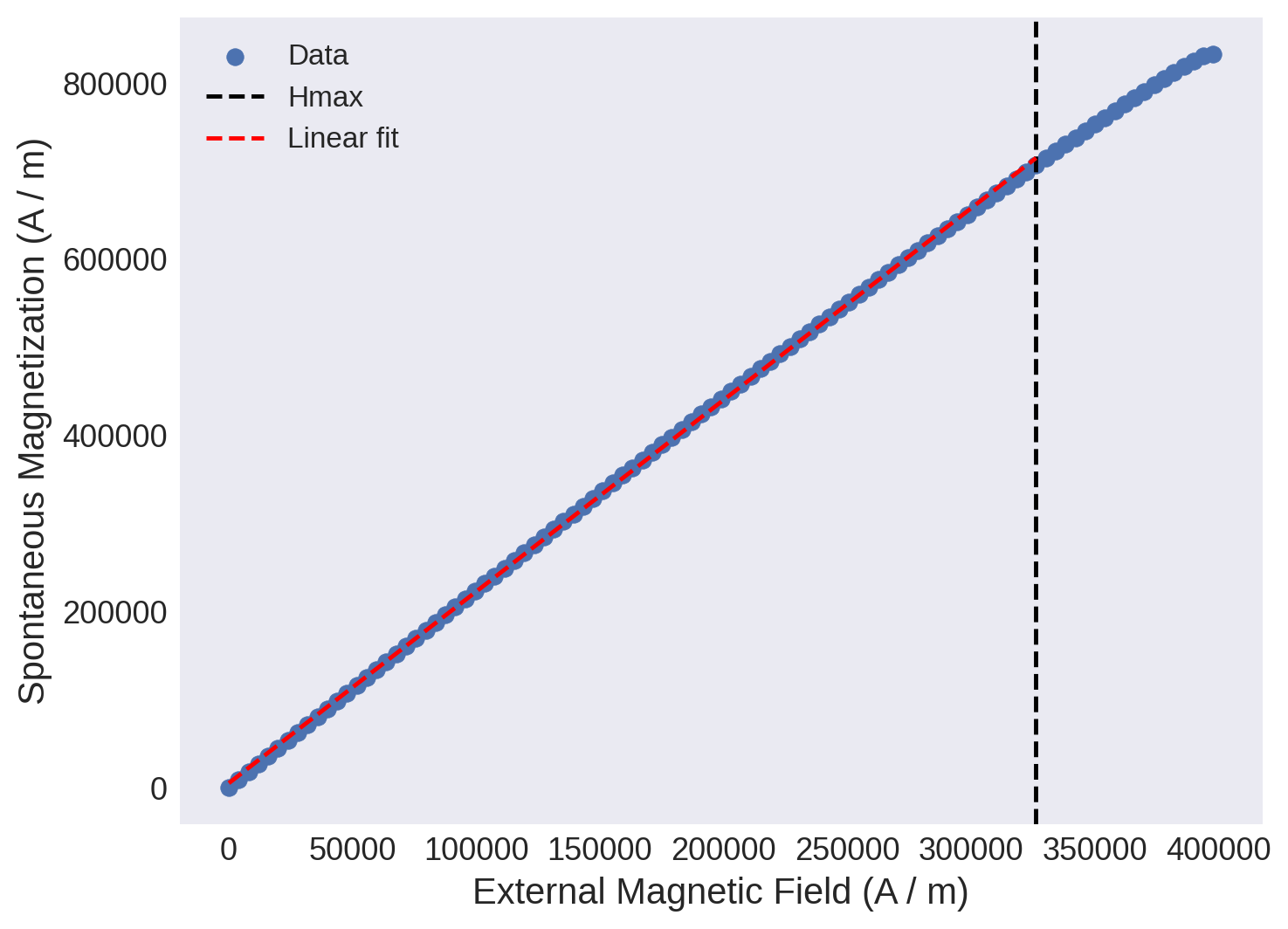
Linear segment#

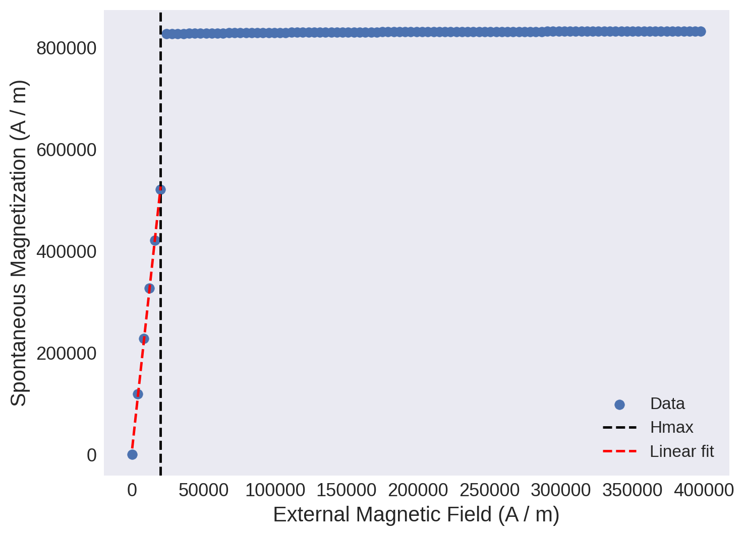
Use mammos-analysis to find the properties of the linearized hysteresis loop.

[20]:

results_linear = mammos_analysis.hysteresis.find_linear_segment(H_y, M_y, margin=0.05 * Ms, min_points=5)

[21]:

results_linear.plot();

../../_images/examples_workflows_sensor_31_0.png

[22]:

results_linear.Hmax  # maximum field value of the linear region

[22]:

ExternalMagneticField(value=19894.36786483437, unit=A / m)

[23]:

results_linear.Mr  # crossing of linear fit and y axis

[23]:

Remanence(value=11682.77113749185, unit=A / m)

[24]:

results_linear.gradient  # slope of the linear fit

[24]:

$25.89454 \; \mathrm{}$

Optimization#

Here we use Bayesian optimization to maximize Hmax by optimizing the lengths of the diagnonals $s_x$ and $s_y$ of the diamond.

[25]:

from bayes_opt import BayesianOptimization

Define the objective function:

[26]:

def objective(sx, sy):
    system.m = df.Field(
        mesh, nvdim=3, value=(1, 0, 0), norm=lambda p: in_diamond(p, sx, sy), valid="norm"
    )  # Change shape
    hd.drive(system, Hsteps=[[Hmin, tuple(Hmax.value), n]], verbose=0)  # Field sweep
    H_y = me.H(system.table.data["By_hysteresis"].values * u.Unit(system.table.units["By_hysteresis"]).to(u.A / u.m))
    M_y = system.table.data["my"].values * Ms
    results_linear = mammos_analysis.hysteresis.find_linear_segment(H_y, M_y, margin=0.05 * Ms, min_points=2)
    return results_linear.Hmax.value

[27]:

objective(19e-9, 39e-9)

[27]:

3978.8735729668742

Running the simulation changes the system so we can view the new shape using:

[28]:

system.m.sel("z").mpl()

../../_images/examples_workflows_sensor_41_0.png

We define the bounds over which the optimizer can search:

[29]:

pbounds = {"sx": (3e-9, np.sqrt(2) * 50e-9), "sy": (3e-9, np.sqrt(2) * 50e-9)}

Initialize the optimizer:

[30]:

optimizer = BayesianOptimization(
    f=objective,
    pbounds=pbounds,
    verbose=2,
    random_state=1,
)

We maximize the objective function:

[31]:

optimizer.maximize(
    init_points=10,
    n_iter=20,
)

|   iter    |  target   |    sx     |    sy     |
-------------------------------------------------
| 1         | 3.979e+03 | 3.124e-08 | 5.177e-08 |
| 2         | 3.979e+03 | 3.008e-09 | 2.347e-08 |
| 3         | 5.173e+04 | 1.294e-08 | 9.252e-09 |
| 4         | 3.979e+03 | 1.561e-08 | 2.64e-08  |
| 5         | 3.979e+03 | 2.987e-08 | 3.948e-08 |
| 6         | 3.979e+03 | 3.138e-08 | 4.94e-08  |
| 7         | 3.979e+03 | 1.684e-08 | 6.246e-08 |
| 8         | 3.979e+03 | 4.854e-09 | 4.84e-08  |
| 9         | 3.979e+03 | 3.126e-08 | 4.083e-08 |
| 10        | 3.979e+03 | 1.251e-08 | 1.641e-08 |
| 11        | 3.979e+05 | 6.878e-08 | 3.093e-09 |
| 12        | 3.979e+05 | 7.033e-08 | 3.693e-09 |
| 13        | 3.979e+05 | 7.042e-08 | 3.294e-09 |
| 14        | 3.979e+05 | 7.051e-08 | 3.277e-09 |
| 15        | 3.979e+05 | 7.065e-08 | 3.624e-09 |
| 16        | 3.979e+05 | 7.022e-08 | 3.215e-09 |
| 17        | 3.979e+05 | 7.007e-08 | 3.54e-09  |
| 18        | 3.979e+05 | 7.06e-08  | 3.728e-09 |
| 19        | 3.382e+05 | 7.051e-08 | 4.495e-09 |
| 20        | 3.979e+05 | 7.012e-08 | 3.568e-09 |
| 21        | 3.979e+05 | 7.025e-08 | 3.039e-09 |
| 22        | 3.86e+05  | 7.06e-08  | 3.868e-09 |
| 23        | 3.74e+05  | 7.063e-08 | 3.973e-09 |
| 24        | 3.979e+05 | 7.068e-08 | 3.728e-09 |
| 25        | 3.979e+05 | 7.018e-08 | 3.468e-09 |
| 26        | 3.979e+05 | 7.062e-08 | 3.572e-09 |
| 27        | 3.979e+05 | 7.029e-08 | 3.141e-09 |
| 28        | 3.143e+05 | 7.054e-08 | 5.716e-09 |
| 29        | 3.979e+05 | 7.043e-08 | 3.014e-09 |
| 30        | 3.979e+05 | 6.98e-08  | 3.234e-09 |
=================================================

[32]:

print(optimizer.max)

{'target': 397887.35729668743, 'params': {'sx': 6.878354081128767e-08, 'sy': 3.092785135534182e-09}}

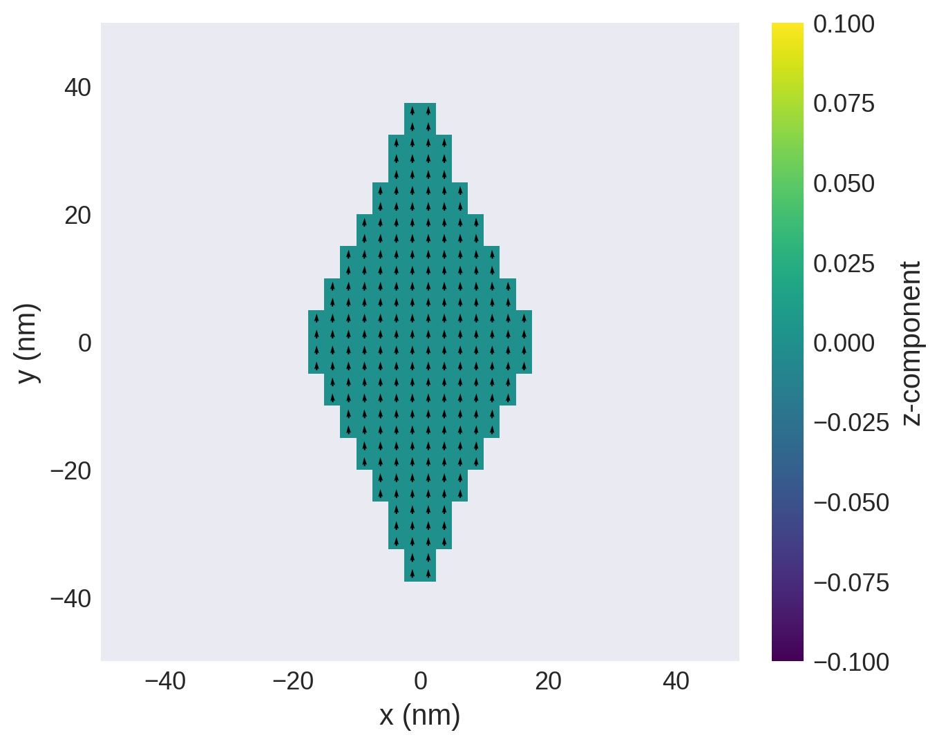
Lets run the simulation again with the best values to check the simulation and the shape.

[33]:

sx, sy = optimizer.max["params"]["sx"], optimizer.max["params"]["sy"]
system.m = df.Field(mesh, nvdim=3, value=(1, 0, 0), norm=lambda p: in_diamond(p, sx, sy), valid="norm")  # Change shape
hd.drive(system, Hsteps=[[Hmin, tuple(Hmax.value), n]], verbose=0)  # Field sweep
H_y = me.H(system.table.data["By_hysteresis"].values * u.Unit(system.table.units["By_hysteresis"]).to(u.A / u.m))
M_y = system.table.data["my"].values * Ms
results_linear = mammos_analysis.hysteresis.find_linear_segment(H_y, M_y, margin=0.01 * Ms, min_points=2)

[34]:

system.m.sel("z").mpl()

../../_images/examples_workflows_sensor_51_0.png

[35]:

results_linear.plot();

../../_images/examples_workflows_sensor_52_0.png

We can also use the built in tools of ubermag to visualize the magnetization as a function of applied field directly.

[36]:

data = md.Data(system.name)

drive = data[-1]

drive.hv(kdims=["x", "y"])

[36]: