mammos_spindynamics quickstart#
mammos_spindynamics provides an interface for working with atomistic spin-dynamics simulations and data.
dbcontains pre-computed temperature-dependent spontaeous magnetization values for several materialsuppasdprovides a Python interface to UppASD
import os
import shutil

import mammos_dft
import mammos_spindynamics

os.environ.setdefault("OMP_NUM_THREADS", "1");  # Use only 1 thread (needed for Binder)
Querying the database – mammos_spindynamics.db#
Use the following function to get a list of all available materials:
mammos_spindynamics.db.find_materials()
| chemical_formula | space_group_name | space_group_number | cell_length_a | cell_length_b | cell_length_c | cell_angle_alpha | cell_angle_beta | cell_angle_gamma | cell_volume | ICSD_label | OQMD_label | source | |
|---|---|---|---|---|---|---|---|---|---|---|---|---|---|
| 0 | Co2Fe2H4 | P6_3/mmc | 194 | 2.645345 Angstrom | 2.645314 Angstrom | 8.539476 Angstrom | 90.0 deg | 90.0 deg | 120.0 deg | 51.751119 Angstrom3 | Uppsala | ||
| 1 | Y2Ti4Fe18 | P4/mbm | 127 | 8.186244 Angstrom | 8.186244 Angstrom | 4.892896 Angstrom | 90.0 deg | 90.0 deg | 90.0 deg | 327.8954234 Angstrom3 | Uppsala | ||
| 2 | Fe16N2 | ? | 0 | 5.680315 Angstrom | 5.680315 Angstrom | 6.2256 Angstrom | 90.0 deg | 90.0 deg | 90.0 deg | 200.875103 Angstrom3 | Uppsala | ||
| 3 | Ni80Fe20 | Pm-3m | 221 | 3.55 Angstrom | 3.55 Angstrom | 3.55 Angstrom | 90.0 deg | 90.0 deg | 90.0 deg | 44.738875 Angstrom3 | https://doi.org/10.48550/arXiv.1908.08885; spa... | ||
| 4 | Fe3Y | 0 | 5.088172 Angstrom | 5.088172 Angstrom | 24.355398 Angstrom | 90.0 deg | 90.0 deg | 120.0 deg | 546.071496 Angstrom3 | Uppsala | |||
| 5 | Fe2.33Ta0.67Y | 0 | 5.227483 Angstrom | 5.227483 Angstrom | 25.022642 Angstrom | 90.0 deg | 90.0 deg | 120.0 deg | 592.173679 Angstrom3 | Uppsala | |||
| 6 | Nd2Fe14B | P42/mnm | 136 | 8.78 Angstrom | 8.78 Angstrom | 12.12 Angstrom | 90.0 deg | 90.0 deg | 90.0 deg | 933.42 Angstrom3 | https://doi.org/10.1103/PhysRevB.99.214409 |
Use the following function to get an object that contains spontaneous magnetization Ms at temperatures T:
results_spindynamics = mammos_spindynamics.db.get_spontaneous_magnetization("Co2Fe2H4")
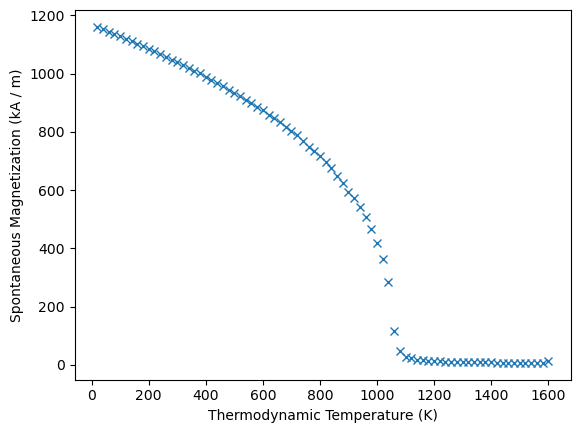
The result object provides a function to plot the data for visual inspection:
results_spindynamics.plot()
<Axes: xlabel='Thermodynamic Temperature (K)', ylabel='Spontaneous Magnetization (kA / m)'>
We can access the Ms and T attributes and get mammos_entity.Entity objects:
results_spindynamics.Ms
[1160.76215153 1152.76454003 1144.33238022 1136.0954238 1128.13437709
1119.86036127 1111.77643794 1102.91850364 1094.39201799 1085.67006372
1076.77881898 1067.42528513 1057.9709741 1048.53821056 1039.91382214
1029.51707701 1019.7181996 1010.21240683 1000.82701767 990.07155621
977.84779712 967.36503405 957.94374674 945.36808824 933.30633679
924.04280638 911.15653709 898.92320851 886.95986875 874.61018656
859.77750325 846.67473396 833.34185235 817.21536597 802.91555665
788.77083768 767.32255016 749.50437039 733.71525356 716.55557269
695.54666554 675.93169422 650.39496667 623.96415571 595.26715472
574.33771381 540.67701871 506.48006839 465.74937929 419.58194399
363.55691471 283.78087533 116.3307659 45.92008375 28.20438383
22.25202686 18.33606449 16.01835637 14.2327736 13.6494969
12.29085695 11.38630509 10.78161436 10.30654019 9.66593883
9.39509234 8.97525861 8.43806344 8.34359373 8.10270528
7.74789847 7.5931119 7.32135685 7.30702274 7.04792251
7.12916484 6.67461312 6.59917726 6.61613203 12.48421016],
unit=kA / m)
results_spindynamics.T
[ 20. 40. 60. 80. 100. 120. 140. 160. 180. 200. 220. 240.
260. 280. 300. 320. 340. 360. 380. 400. 420. 440. 460. 480.
500. 520. 540. 560. 580. 600. 620. 640. 660. 680. 700. 720.
740. 760. 780. 800. 820. 840. 860. 880. 900. 920. 940. 960.
980. 1000. 1020. 1040. 1060. 1080. 1100. 1120. 1140. 1160. 1180. 1200.
1220. 1240. 1260. 1280. 1300. 1320. 1340. 1360. 1380. 1400. 1420. 1440.
1460. 1480. 1500. 1520. 1540. 1560. 1580. 1600.],
unit=K)
To work with the data we can also get it as pandas.DataFrame. The dataframe only contains the values (not units).
results_spindynamics.dataframe
| T | Ms | |
|---|---|---|
| 0 | 20.0 | 1160.762152 |
| 1 | 40.0 | 1152.764540 |
| 2 | 60.0 | 1144.332380 |
| 3 | 80.0 | 1136.095424 |
| 4 | 100.0 | 1128.134377 |
| ... | ... | ... |
| 75 | 1520.0 | 7.129165 |
| 76 | 1540.0 | 6.674613 |
| 77 | 1560.0 | 6.599177 |
| 78 | 1580.0 | 6.616132 |
| 79 | 1600.0 | 12.484210 |
80 rows × 2 columns
Running spindynamics simulations – mammos_spindynamics.uppasd#
The uppasd subpackage provides an Python interface to UppASD (the Uppsala Atomistic Spin Dynamics Software). UppASD has to be installed separately and the executable must be in your PATH. The easiest way is to install UppASD from conda-forge using pixi or conda.
In this notebook we will show how to run a single simulation. We assume that we have all required input files. The uppasd notebook will explain both creating inputs as well as analyzing the resulting data in more detail.
We will run a simulation for Co2Fe2H4. We can get three of the required input files for this material from mammos_dft.db:
exchangecontaining the exchange coupling constants \(J_{ij}\)posfilecontaining the position of the atoms in the unit cellmomfilecontaining the magnetic moments of the atoms in the unit cell
We will first copy the three files to the current directory. This most closely resembles the scenario where you may have your own files. We will also rename exchange to jfile (for no good reason, just to show that we can) and use that name in inpsd.dat further down.
In practice, you should avoid this manual copy when using files from the database in mammos_dft and instead pass the paths to the three files as additional keyword arguments when creating the simulation object, as explained in the uppasd notebook.
To access the data files coming with mammos_dft.db we use the get_uppasd_properties function:
uppasd_inputs = mammos_dft.db.get_uppasd_properties("Co2Fe2H4")
The returned object gives access to the available files, e.g.:
uppasd_inputs.posfile
PosixPath('/home/runner/work/mammos/mammos/.pixi/envs/docs/lib/python3.11/site-packages/mammos_dft/data/Co2Fe2H4/posfile')
# copy files to simulate that we have our own files
shutil.copy(uppasd_inputs.posfile, ".")
shutil.copy(uppasd_inputs.momfile, ".")
shutil.copy(uppasd_inputs.exchange, "./jfile");
In addition we have to create the main input file inpsd.dat. For detailed documentation about this file and UppASD in general refer to the UppASD documentation.
In this notebook we create the file using the writefile magic, as a user you may already have your own input file, which you can use.
Warning
In order to keep the runtime of this notebook short we use unreasonably small values for ncell, ip_mcnstep and mcnstep.
For production runs you will have to use higher values, suitable starting points could be ncell 32 32 32, ip_mcnstep 25000, mcnstep 50000
%%writefile inpsd.dat
simid Co2Fe2H4

cell  1.000000000000000  -0.500000000182990   0.000000000000000
      0.000000000000000   0.866011964524435   0.000000000000000
      0.000000000000000   0.000000000000000   3.228114436804486

ncell 12  12  12
bc    P P P
sym 0
posfile ./posfile
posfiletype D

initmag 3
momfile ./momfile
maptype 2
exchange ./jfile
ip_mode M
ip_temp 20
ip_mcnstep 200

mode M
temp 20
mcnstep 200
plotenergy 1
do_proj_avrg Y
do_cumu Y

alat 2.6489381562e-10
Writing inpsd.dat
We pass the input file paths together with paths to the other three files to the Simulation class:
sim = mammos_spindynamics.uppasd.Simulation(inpsd="inpsd.dat")
We can now use this object to run a simulation. We need to pass a path to a directory where the output will be written to. Optionally, we can also pass a human-readable description, which will be saved as additional metadata.
result = sim.run(out="Co2Fe2H4-short", description="Short test for Co2Fe2H4")
Running UppASD in Co2Fe2H4-short/0-run ...
simulation finished, took 0:00:07
We get an object back, which allows us to inspect simulation output:
result.T
result.Ms
result.Cv
We can also access some simulation metadata, e.g. the description and the runtime:
result.info()
| name | description | time_elapsed | |
|---|---|---|---|
| 0 | 0-run | Short test for Co2Fe2H4 | 0:00:07 |