mammos_analysis quickstart

mammos_analysis has a collection of post-processing tools:

• mammos_analysis.hysteresis contains functions to extract macroscopic properties from a hysteresis loop

• mammos_analysis.kuzmin contains fuctions to estimate micromagnetic properties from (atomistic) M(T) data using Kuz’min equations.

import mammos_analysis
import mammos_entity as me
import mammos_units as u
import numpy as np

import matplotlib.pyplot as plt

mammos_analysis.hysteresis

Extrinsic properties Hc, Mr, BHmax

We can compute coercive field Hc, remanent magnetization Mr and the maximum energy product BHmax from a hysteresis loop.

We need to provide the external field H and the magnetization M. These could come from a simulation or experiment. Here, we create some artificial data:

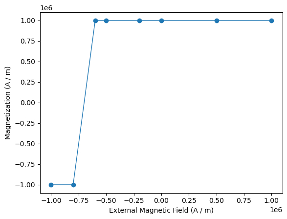
H = me.H([-1e6, -0.5e6, -0.2e6, 0, 0.5e6, 1e6])
M = me.M([-1e6, -1e6, 1e6, 1e6, 1e6, 1e6])
plt.plot(H.q, M.q, "o-", linewidth=1)

[<matplotlib.lines.Line2D at 0x7f552eebebd0>]

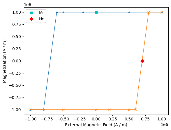
extrinsic_properties = mammos_analysis.hysteresis.extrinsic_properties(
    H=H,
    M=M,
    demagnetization_coefficient=1 / 3,  # assumption: we have a cube
)

extrinsic_properties.Mr

Remanence(value=1000000.0, unit=A / m)

extrinsic_properties.Hc

CoercivityHcExternal(value=350000.0, unit=A / m)

extrinsic_properties.BHmax  # only available if we pass a demagnetization_coefficient, otherwise NaN

MaximumEnergyProduct(value=117286.12579786668, unit=A T / m)

plt.plot(H.q, M.q, ".-", -H.q, -M.q, "x-", linewidth=1)
plt.plot(0, extrinsic_properties.Mr.q, "cs", label="Mr")
plt.plot(extrinsic_properties.Hc.q, 0, "rD", label="Hc")
plt.legend()

<matplotlib.legend.Legend at 0x7f552ccb9790>

Linear segment of a hysteresis loop

We can compute properties the linear segment (starting at H=0) of a hysteresis loop.

We need to provide the external field H and the magnetization M. These could come from a simulation or experiment. Here, we create some artificial data:

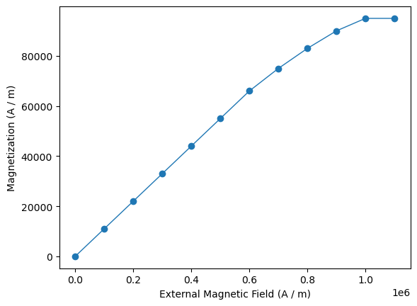
H = me.H(np.linspace(0, 1.1e6, 12))
M = me.M([0, 0.11e5, 0.22e5, 0.33e5, 0.44e5, 0.55e5, 0.66e5, 0.75e5, 0.83e5, 0.90e5, 0.95e5, 0.95e5])
plt.plot(H.q, M.q, "o-", linewidth=1)

[<matplotlib.lines.Line2D at 0x7f552cb8df90>]

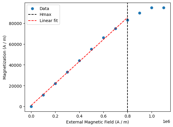
margin = 0.03 * 0.95e5  # allow 3% maximum deviation from assumed Ms=0.95e5
linear_segment_properties = mammos_analysis.hysteresis.find_linear_segment(H=H, M=M, margin=margin, min_points=3)

linear_segment_properties.plot()

<Axes: xlabel='External Magnetic Field (A / m)', ylabel='Spontaneous Magnetization (A / m)'>

mammos_analysis.kuzmin

Functionality to extract estimated micromagnetic properties from Ms(T) data, which could e.g. come from spin dynamics simulations.

• We use Kuz’min equations to compute Ms(T), A(T), K1(T)

• Kuz’min, M.D., Skokov, K.P., Diop, L.B. et al. Exchange stiffness of ferromagnets. Eur. Phys. J. Plus 135, 301 (2020). https://doi.org/10.1140/epjp/s13360-020-00294-y

• Additional details about inputs and outputs are available in the API reference

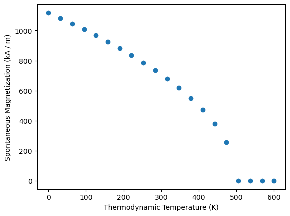
In this notebook we will use artificial data:

T = me.T(np.linspace(0, 600, 20))
Ms_val = np.sqrt(500 - T.value, where=T.value < 500, out=np.zeros_like(T.value)) * 0.5e5
Ms = me.Ms(Ms_val)
plt.plot(T.q, Ms.q, "o")

[<matplotlib.lines.Line2D at 0x7f552cc17750>]

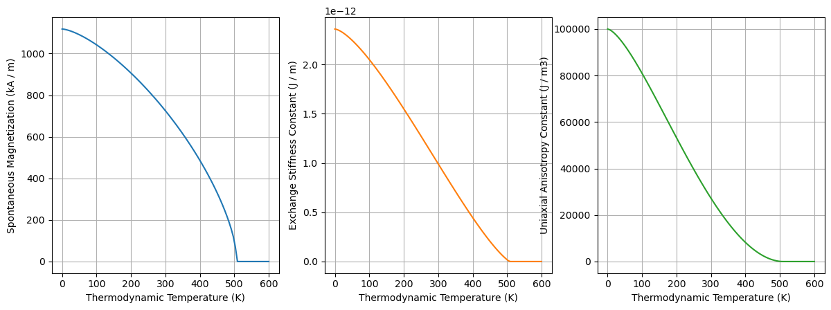
kuzmin_result = mammos_analysis.kuzmin.kuzmin_properties(T=T, Ms=Ms, K1_0=1e5)  # K1_0 is optional

We can visualize the resulting functions and compare against our input data:

kuzmin_result.plot()

array([<Axes: xlabel='Thermodynamic Temperature (K)', ylabel='Spontaneous Magnetization (A / m)'>,
       <Axes: xlabel='Thermodynamic Temperature (K)', ylabel='Exchange Stiffness Constant (J / m)'>,
       <Axes: xlabel='Thermodynamic Temperature (K)', ylabel='Uniaxial Anisotropy Constant (J / m3)'>],
      dtype=object)

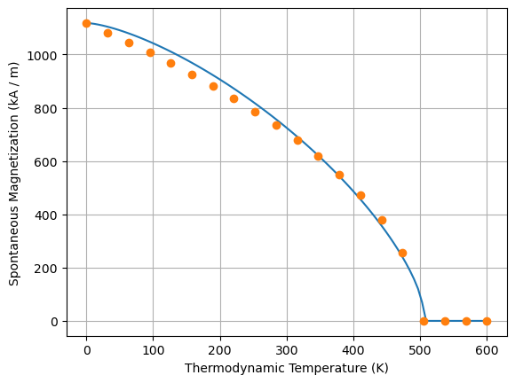
kuzmin_result.Ms.plot()
plt.plot(T.q, Ms.q, "o")

[<matplotlib.lines.Line2D at 0x7f555d4bb590>]

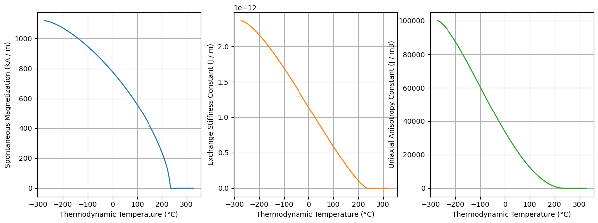
We can also generate these plots using temperature in degree Celsius by using the celsius argument:

kuzmin_result.plot(celsius=True);

The result object contains three functions for Ms, A, and K1. K1 is only available if we pass K1_0 to the kuzmin_properties function. Furthermore, we get an estimated Curie temperature and the fit parameter s.

kuzmin_result

KuzminResult(Ms=Ms(T), A=A(T), Tc=Entity(ontology_label='CurieTemperature', value=np.float64(511.0022776647576), unit='K'), s=<Quantity 2.52133756>, K1=K1(T))

We can call the functions at different temperatures to get parameters. We can pass a mammos_entity.Entity, an astropy.units.Quantity or a number:

kuzmin_result.Ms(me.T(0))

SpontaneousMagnetization(value=1118033.988749895, unit=A / m)

kuzmin_result.A(100 * u.K)

ExchangeStiffnessConstant(value=2.032233964260887e-12, unit=J / m)

kuzmin_result.K1(300)

UniaxialAnisotropyConstant(value=26759.335152727293, unit=J / m3)

We can also use an array to get data for multiple temperatures:

kuzmin_result.Ms(me.T([0, 100, 200, 300]))

SpontaneousMagnetization(value=[1118033.9887499  1041124.93901139  903894.36591862  720465.92637849], unit=A / m)