Hard magnet tutorial#
Introduction#
In this notebook we explore hard magnet properties such as Hc as function of temperature for Fe16N2.
We query databases to get temperature-dependent inputs for micromagnetic simulations from DFT and spin dynamics simulations
We run hysteresis simulations and compute derived quantities.
Requirements:
Software:
mammos,esys-escriptBasic understanding of mammos-units and mammos-entity
The MODA diagram is provided at the bottom of the notebook.
%config InlineBackend.figure_format = "retina"

import math

import mammos_analysis
import mammos_dft
import mammos_entity as me
import mammos_mumag
import mammos_spindynamics
import mammos_units as u
import matplotlib.pyplot as plt
import numpy as np
import pandas as pd
from matplotlib import colormaps
# Allow convenient conversions between A/m and T
u.set_enabled_equivalencies(u.magnetic_flux_field());
DFT data: magnetization and anisotropy at zero Kelvin#
The first step loads spontaneous magnetization Ms_0 and the uniaxial anisotropy constant K1_0 from a database of DFT calculations (at T=0K).
We can use the print_info flag to trigger printing of crystallographic information.
material = "Fe2.33Ta0.67Y"

results_dft = mammos_dft.db.get_micromagnetic_properties(material, print_info=True)
Found material in database.
Chemical Formula: Fe2.33Ta0.67Y
Space group name:
Space group number: 0
Cell length a: 5.227483 Angstrom
Cell length b: 5.227483 Angstrom
Cell length c: 25.022642 Angstrom
Cell angle alpha: 90.0 deg
Cell angle beta: 90.0 deg
Cell angle gamma: 120.0 deg
Cell volume: 592.173679 Angstrom3
ICSD_label:
OQMD_label:
results_dft
MicromagneticProperties(Ms_0=Entity(ontology_label='SpontaneousMagnetization', value=612746.0, unit='A / m'), Ku_0=Entity(ontology_label='UniaxialAnisotropyConstant', value=2170000.0, unit='J / m3'))
results_dft.Ms_0
results_dft.Ku_0
Temperature-dependent magnetization data from spindynamics database lookup#
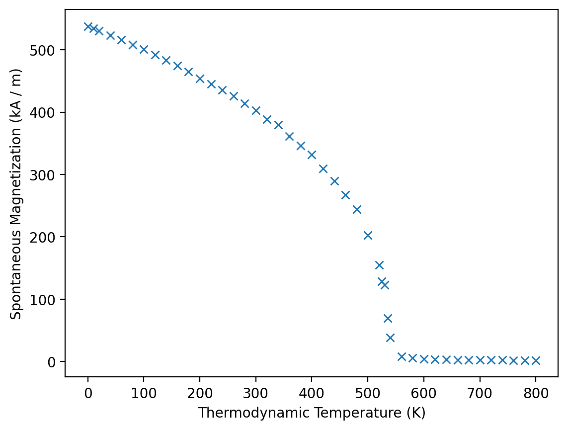
In the second step we use a spin dynamics calculation database to load data for the temperature-dependent magnetization.
results_spindynamics = mammos_spindynamics.db.get_spontaneous_magnetization(material)
We can visualize the pre-computed data using .plot.
results_spindynamics.plot();
We can access T and Ms and get mammos_entity.Entity objects:
results_spindynamics.T
[ 0. 10. 20. 40. 60. 80. 100. 120. 140. 160. 180. 200. 220. 240.
260. 280. 300. 320. 340. 360. 380. 400. 420. 440. 460. 480. 500. 520.
525. 530. 535. 540. 560. 580. 600. 620. 640. 660. 680. 700. 720. 740.
760. 780. 800.],
unit=K)
results_spindynamics.Ms
[537.69407444 534.21010153 530.76436753 523.25014179 515.73821821
508.25887022 500.54039671 492.13118265 483.75561632 474.76662259
465.11579689 454.00477917 445.20747657 435.9139003 425.91795755
414.30225011 402.86923234 388.78720606 379.37938009 361.08960761
346.18346011 331.51212323 309.32538618 289.79102668 267.5673475
244.08728601 203.11783041 154.86746066 128.5319578 123.41379485
69.79521779 38.60654427 8.52781909 5.67183537 4.5456332
3.69262584 3.23444053 2.93970208 2.71010548 2.57155219
2.3322868 2.28983246 2.16204657 2.06734541 2.00064899],
unit=kA / m)
We can get also the data in the form of a pandas.DataFrame, which only contains the values in SI units:
results_spindynamics.dataframe.head()
| T | Ms | |
|---|---|---|
| 0 | 0.0 | 537.694074 |
| 1 | 10.0 | 534.210102 |
| 2 | 20.0 | 530.764368 |
| 3 | 40.0 | 523.250142 |
| 4 | 60.0 | 515.738218 |
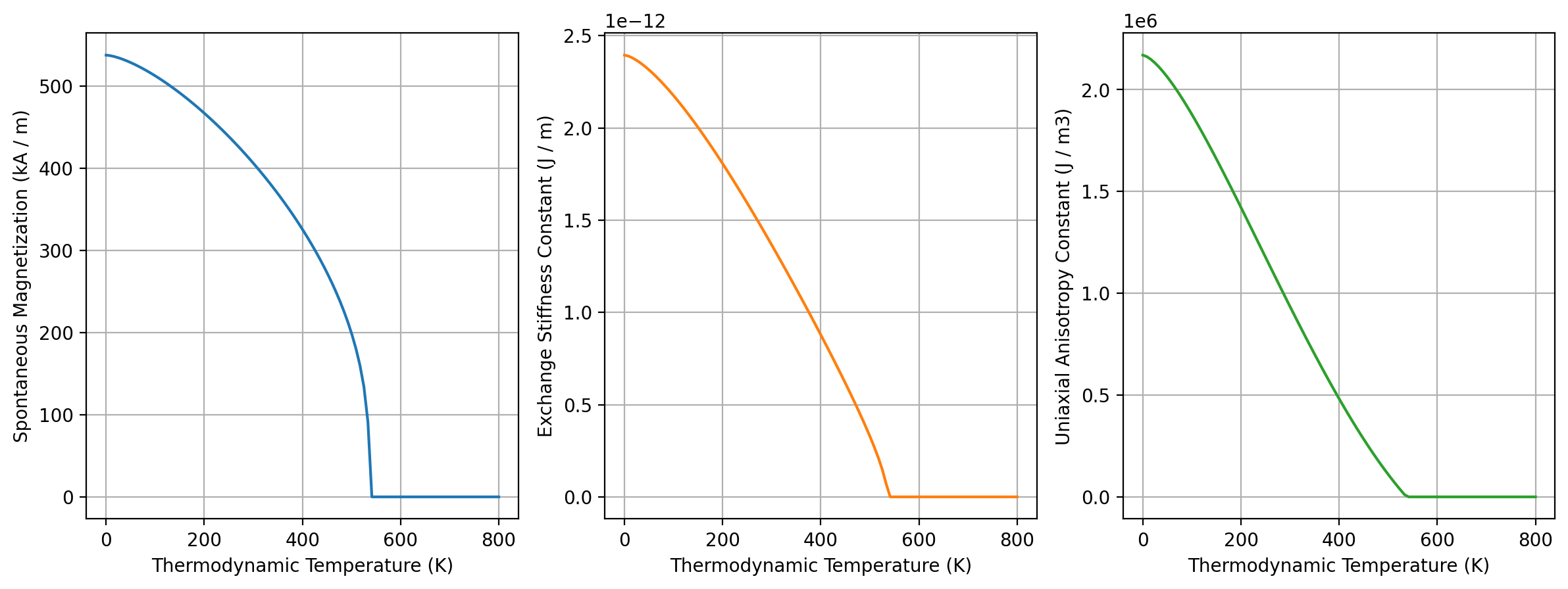
Calculate micromagnetic intrinsic properties using Kuz’min formula#
We use Kuz’min equations to compute Ms(T), A(T), K1(T)
Kuz’min, M.D., Skokov, K.P., Diop, L.B. et al. Exchange stiffness of ferromagnets. Eur. Phys. J. Plus 135, 301 (2020). https://doi.org/10.1140/epjp/s13360-020-00294-y
Additional details about inputs and outputs are available in the API reference
results_kuzmin = mammos_analysis.kuzmin_properties(
    T=results_spindynamics.T,
    Ms=results_spindynamics.Ms,
    K1_0=results_dft.Ku_0,
)
The plot method of the returned object can be used to visualize temperature-dependence of all three quantities. The temperature range matches that of the fit data:
results_kuzmin.plot();
results_kuzmin
KuzminResult(Ms=Ms(T), A=A(T), Tc=Entity(ontology_label='CurieTemperature', value=537.1888739138071, unit='K'), s=<Quantity 1.82478153>, K1=K1(T))
The attributes
Ms,AandK1provide fit results as function of temperature. They each have aplotmethod.Tcis the fitted Curie temperature.sis a fit parameter in the Kuzmin equation.
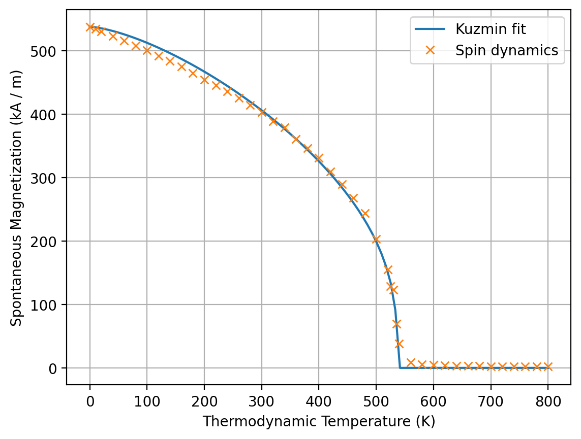
To visually assess the accuracy of the fit, we can combine the plot methods of results_kuzmin.Ms and results_spindynamics:
ax = results_kuzmin.Ms.plot(label="Kuzmin fit")
results_spindynamics.plot(ax=ax, label="Spin dynamics");
To get inputs for the micromagnetic simulation at a specific temperature we call the three attributes Ms, A and K1. We can pass a mammos_entity.Entity, an astropy.units.Quantity or a number:
temperature = me.T(300)
temperature
results_kuzmin.Ms(temperature) # Evaluation with Entity
results_kuzmin.A(300 * u.K) # Evaluation with Quantity
results_kuzmin.K1(300) # Evaluation with number
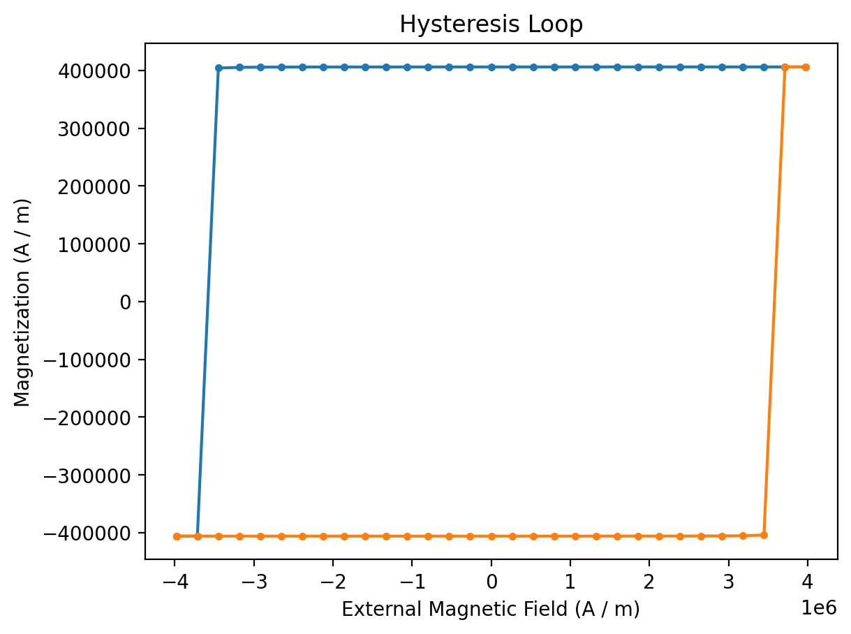
Run micromagnetic simulation to compute hysteresis loop#
We now compute a hysteresis loop (using a finite-element micromagnetic simulation) with the material parameters we have obtained.
We simulate a 20x20x20 nm cube for which a pre-defined mesh is available.
Additional documentation of this step is available this notebook.
results_hysteresis = mammos_mumag.hysteresis.run(
    mesh="cube20_singlegrain_msize2",
    Ms=results_kuzmin.Ms(temperature),
    A=results_kuzmin.A(temperature),
    K1=results_kuzmin.K1(temperature),
    theta=0,
    phi=0,
    h_start=(5 * u.T).to(u.A / u.m),
    h_final=(-5 * u.T).to(u.A / u.m),
    h_n_steps=30,
)
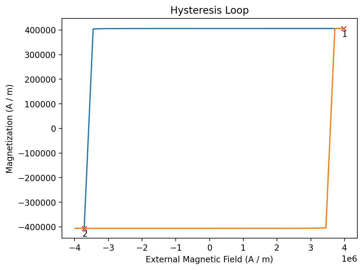
The returned results_hysteresis object provides a plot method to visualize the computed data. mammos_mumag.hysteresis only computes half a hysteresis loop, going from h_start to h_final. To show a full loop this function mirrors the computed data and plots it twice:
results_hysteresis.plot(marker="."); # blue: simulation output, orange: mirrored data
The result object provides access to H and M:
results_hysteresis.H
[ 3.97887358e+06 3.71361534e+06 3.44835710e+06 3.18309886e+06
2.91784062e+06 2.65258238e+06 2.38732415e+06 2.12206591e+06
1.85680767e+06 1.59154943e+06 1.32629119e+06 1.06103295e+06
7.95774715e+05 5.30516477e+05 2.65258238e+05 2.65046223e-10
-2.65258238e+05 -5.30516477e+05 -7.95774715e+05 -1.06103295e+06
-1.32629119e+06 -1.59154943e+06 -1.85680767e+06 -2.12206591e+06
-2.38732415e+06 -2.65258238e+06 -2.91784062e+06 -3.18309886e+06
-3.44835710e+06 -3.71361534e+06 -3.97887358e+06],
unit=A / m)
results_hysteresis.M
[ 406047.45956514 406046.92223571 406046.32676674 406045.66444942
406044.92487697 406044.09552231 406043.16123259 406042.10347411
406040.89945688 406039.52086091 406037.93214617 406036.08822693
406033.93125809 406031.38592987 406028.35281696 406024.6984277
406020.24013677 406014.72273337 406007.7806909 405998.87542387
405987.18632141 405971.41226388 405949.38763287 405917.28359447
405867.78611011 405785.3957462 405632.02921316 405289.18253948
404149.88495849 -406046.92212471 -406047.45959509],
unit=A / m)
The dataframe property generates a dataframe in the SI units.
results_hysteresis.dataframe.head()
| configuration_type | H | M | Mx | My | Mz | energy_density | |
|---|---|---|---|---|---|---|---|
| 0 | 1 | 3.978874e+06 | 406047.459565 | -4.121685 | -8.621428 | 406047.459565 | -2.933988e+06 |
| 1 | 1 | 3.713615e+06 | 406046.922236 | -4.270307 | -8.929829 | 406046.922236 | -2.798639e+06 |
| 2 | 1 | 3.448357e+06 | 406046.326767 | -4.430020 | -9.260933 | 406046.326767 | -2.663290e+06 |
| 3 | 1 | 3.183099e+06 | 406045.664449 | -4.602162 | -9.617560 | 406045.664449 | -2.527941e+06 |
| 4 | 1 | 2.917841e+06 | 406044.924877 | -4.788244 | -10.002779 | 406044.924877 | -2.392593e+06 |
We can generate a table in alternate units:
df = pd.DataFrame(
    {
        "mu0_H": results_hysteresis.H.q.to(u.T),
        "J": results_hysteresis.M.q.to(u.T),
    },
)
df.head()
| mu0_H | J | |
|---|---|---|
| 0 | 5.000000 | 0.510254 |
| 1 | 4.666667 | 0.510254 |
| 2 | 4.333333 | 0.510253 |
| 3 | 4.000000 | 0.510252 |
| 4 | 3.666667 | 0.510251 |
Plotting of magnetization configurations#
Simulation stores specific magnetization field configurations:
results_hysteresis.plot(configuration_marks=True);
results_hysteresis.configurations
{1: PosixPath('/tmp/tmpi2gk9qp_/hystloop/hystloop_0001.vtu'),
 2: PosixPath('/tmp/tmpi2gk9qp_/hystloop/hystloop_0002.vtu')}
# results_hysteresis.plot_configuration(1);
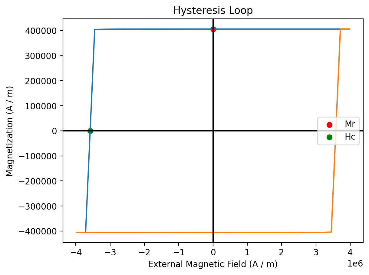
Analyze hysteresis loop#
We can extract extrinsic properties with the extrinsic_properties function from the mammos_analysis package:
extrinsic_properties = mammos_analysis.hysteresis.extrinsic_properties(
    results_hysteresis.H,
    results_hysteresis.M,
    demagnetization_coefficient=1 / 3,
)
/home/runner/work/mammos/mammos/.pixi/envs/docs/lib/python3.11/site-packages/mammos_analysis/hysteresis.py:382: UserWarning: Only 2 (H_internal, M_internal) values in second quadrant - estimate of BHmax may be inaccurate.
  warnings.warn(
extrinsic_properties.Hc
extrinsic_properties.Mr
extrinsic_properties.BHmax
We can combine the results_hysteresis.plot method with some custom code to show Hc and Mr in the hysteresis plot:
ax = results_hysteresis.plot()
ax.scatter(0, extrinsic_properties.Mr.value, c="r", label="Mr")
ax.scatter(-extrinsic_properties.Hc.value, 0, c="g", label="Hc")
ax.axhline(0, c="k")  # Horizontal line at M=0
ax.axvline(0, c="k")  # Vertical line at H=0
ax.legend();
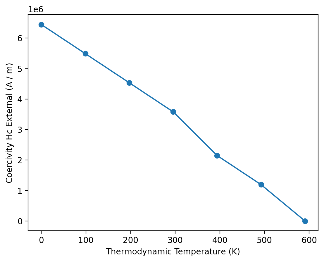
Compute Hc(T)#
We can leverage mammos to calculate Hc(T) for multiple values of T.
First, we run hysteresis simulations at 7 different temperatures and collect all simulation results:
T = np.linspace(0, 1.1 * results_kuzmin.Tc.q, 7)

simulations = []
for temperature in T:
    print(f"Running simulation for T={temperature:.0f}")
    results_hysteresis = mammos_mumag.hysteresis.run(
        mesh="cube20_singlegrain_msize2",
        Ms=results_kuzmin.Ms(temperature),
        A=results_kuzmin.A(temperature),
        K1=results_kuzmin.K1(temperature),
        theta=0,
        phi=0,
        h_start=(9 * u.T).to(u.A / u.m),
        h_final=(-9 * u.T).to(u.A / u.m),
        h_n_steps=30,
    )
    simulations.append(results_hysteresis)
Running simulation for T=0 K
Running simulation for T=98 K
Running simulation for T=197 K
Running simulation for T=295 K
Running simulation for T=394 K
Running simulation for T=492 K
Running simulation for T=591 K
We can now use mammos_analysis.hysteresis as shown before to extract Hc for all simulations and visualize Hc(T):
Hcs = []
for res in simulations:
    cf = mammos_analysis.hysteresis.extract_coercive_field(H=res.H, M=res.M).value
    if np.isnan(cf):  # Above Tc
        cf = 0
    Hcs.append(cf)
plt.plot(T, Hcs, linestyle="-", marker="o")
plt.xlabel(me.T().axis_label)
plt.ylabel(me.Hc().axis_label);
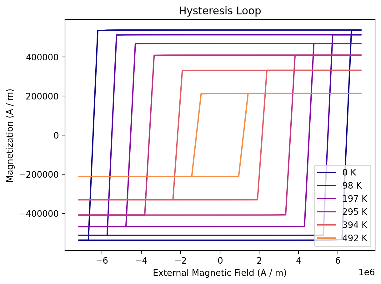
We can also show the hysteresis loops of all simulations:
colors = colormaps["plasma"].colors[:: math.ceil(256 / len(T))]

fix, ax = plt.subplots()
for temperature, sim, color in zip(T, simulations, colors, strict=False):
    if np.isnan(sim.M.q).all():  # no Ms above Tc
        continue
    sim.plot(ax=ax, label=f"{temperature:.0f}", color=color, duplicate_change_color=False)
ax.legend(loc="lower right");
MODA for the workflow#
