Sensor shape optimization workflow#
In this example we will show how to use MaMMoS for shape optimization of a magnetic sensor element. To show the versatility of the mammos software we will perform the micromagnetic simulations with the ubermag micromagnetic package.
In this workflow we optimize the region of the hysteresis loop over which M vs H has a linear reponse. In order to do this we will first obtain micromagnetic parameters, perform micromagnetic simulations, and then analyze the hysteresis loop.
This is followed by Bayesian optimization to maximize the linear region.
Requirements:
Software:
mammos,ubermagwith OOMMF,bayesian-optimizationBasic understanding of mammos-units and mammos-entity
The MODA diagram is provided at the bottom of the notebook.
%config InlineBackend.figure_format = "retina"

# MaMMoS imports
# Ubermag imports
import discretisedfield as df
import mammos_analysis
import mammos_entity as me
import mammos_spindynamics
import mammos_units as u
import micromagneticdata as md
import micromagneticmodel as mm
import numpy as np
import oommfc as mc
%config InlineBackend.figure_format = "retina"
# Allow convenient conversions between A/m and T
u.set_enabled_equivalencies(u.magnetic_flux_field());
Temperature-dependent magnetization data from spindynamics database lookup#
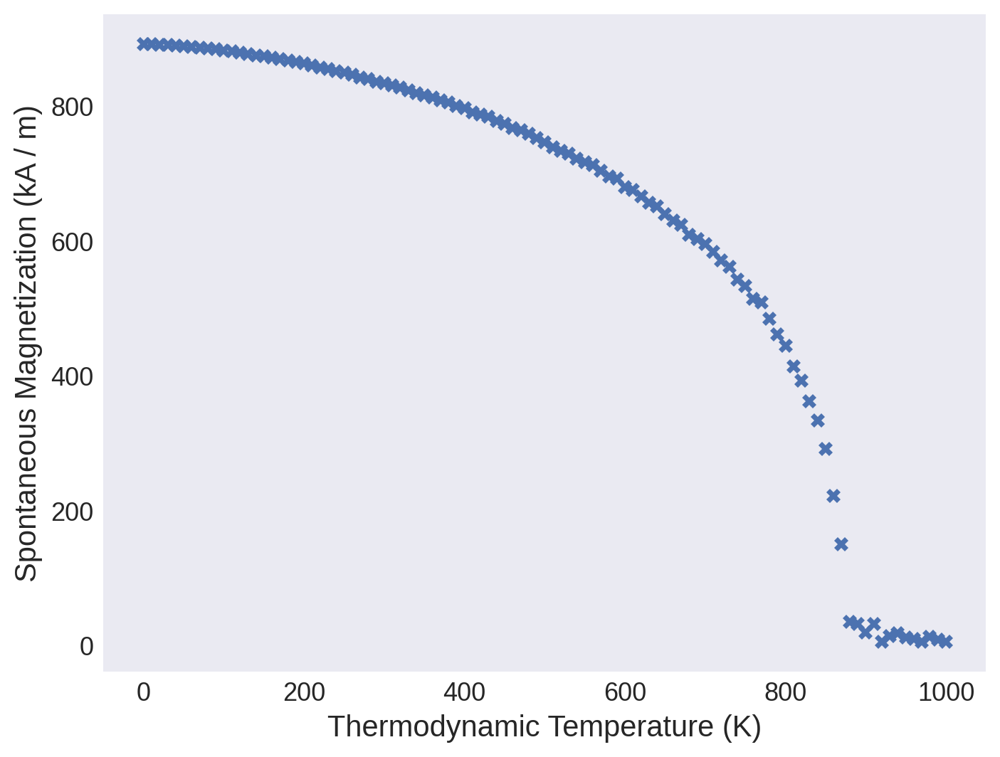
In order to get micromagnetic parameters we use pre-computed data from mammos_spindynamics.db for the temperature-dependent magnetization.
results_spindynamics = mammos_spindynamics.db.get_spontaneous_magnetization("Ni80Fe20")
We can visualize the pre-computed data using .plot.
results_spindynamics.plot(marker="X");
We can access T and Ms and get mammos_entity.Entity objects:
results_spindynamics.T
[ 0. 10. 20. 30. 40. 50. 60. 70. 80. 90. 100. 110.
120. 130. 140. 150. 160. 170. 180. 190. 200. 210. 220. 230.
240. 250. 260. 270. 280. 290. 300. 310. 320. 330. 340. 350.
360. 370. 380. 390. 400. 410. 420. 430. 440. 450. 460. 470.
480. 490. 500. 510. 520. 530. 540. 550. 560. 570. 580. 590.
600. 610. 620. 630. 640. 650. 660. 670. 680. 690. 700. 710.
720. 730. 740. 750. 760. 770. 780. 790. 800. 810. 820. 830.
840. 850. 860. 870. 880. 890. 900. 910. 920. 930. 940. 950.
960. 970. 980. 990. 1000.],
unit=K)
results_spindynamics.Ms
[892.18469121 891.9696747 891.51376832 890.89459215 890.08359626
889.19944123 888.17164447 887.05373705 885.67174297 884.39591886
883.07994644 881.49542643 879.78867711 877.78839903 875.83451456
874.08137164 872.0498671 869.91219258 867.44262535 865.56279221
863.20920899 860.45771141 857.76331364 855.29642297 852.46641313
849.52398802 846.41472437 842.90486979 840.14891128 836.73452047
833.91878558 830.96386988 827.69133644 824.07174315 819.58405415
816.18750703 812.56523718 809.16869006 805.46612359 800.4654284
796.73341984 791.03682058 787.26823245 784.89412898 777.77181859
774.07371305 767.97295413 764.32837967 758.78612837 752.67377105
746.86743308 739.28743194 734.19484172 730.16841221 722.19584981
716.59828306 712.64322832 704.57609434 696.4018982 692.47093245
680.04993718 676.43837355 666.86344745 656.97536451 651.92738353
640.06400369 630.1562927 624.16081157 609.41924392 603.3648786
595.3343242 584.19182959 572.02153822 561.56424145 543.28426931
533.35782244 514.57733469 508.8941182 485.02996208 462.14988568
445.50439589 414.82127218 393.52036268 363.20838779 334.08391073
292.25829241 222.77316429 150.43215297 36.09056591 32.87468619
19.76385372 32.64120146 6.22241722 14.94480733 18.46081798
12.18688601 10.18393138 6.62918207 13.1756943 9.66914081
6.27331636],
unit=kA / m)
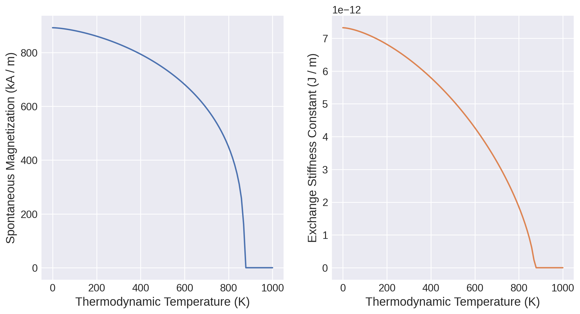
Calculate micromagnetic intrinsic properties using Kuz’min formula#
We use Kuz’min equations to compute Ms(T) and A(T).
kuzmin_result = mammos_analysis.kuzmin_properties(
    T=results_spindynamics.T,
    Ms=results_spindynamics.Ms,
)
kuzmin_result.plot();
kuzmin_result
KuzminResult(Ms=Ms(T), A=A(T), Tc=Entity(ontology_label='CurieTemperature', value=871.9217838428029, unit='K'), s=<Quantity 0.90900525>, K1=None)
kuzmin_result.Ms(0)
kuzmin_result
KuzminResult(Ms=Ms(T), A=A(T), Tc=Entity(ontology_label='CurieTemperature', value=871.9217838428029, unit='K'), s=<Quantity 0.90900525>, K1=None)
kuzmin_result.Ms(0)
Setting up the micromagnetic simulation#
Run the micromagnetic simulation with parameters at 300 K using ubermag with OOMMF as calculator.
T = me.T(300, unit="K")
Define the energy equation of the system.
system = mm.System(name="sensor")
A = kuzmin_result.A(T)
Ms = kuzmin_result.Ms(T)
system.energy = mm.Exchange(A=A.value) + mm.Demag() + mm.Zeeman(H=(0, 0, 0))
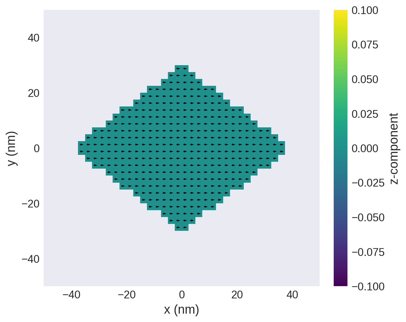
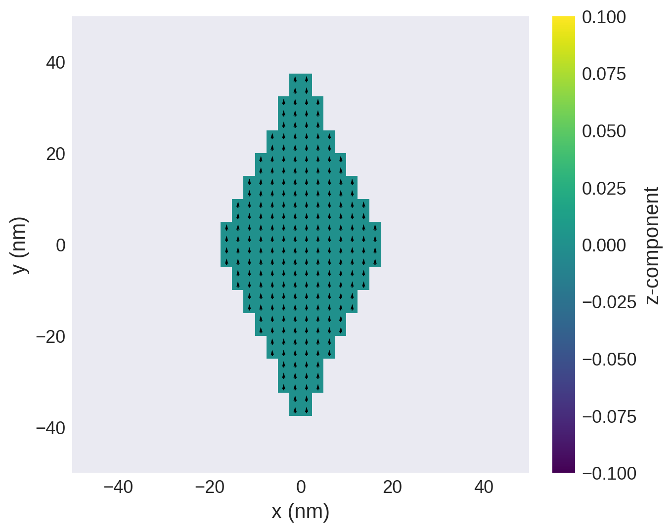
Initialize the magnetization: we constrain the shape of our sensor to be a diamond (rhombus) with the distance \(s_x\) and \(s_y\) from origin to corners along the \(x\) and \(y\) directions, respectively, and with thickness \(t\). We create a \(100\times 100\times 5\) nm region in which we create the diamond shape of magnetic material.
L = 100e-9  # nm
t = 5e-9  # nm
region = df.Region(p1=(-L / 2, -L / 2, -t / 2), p2=(L / 2, L / 2, t / 2))
mesh = df.Mesh(region=region, n=(40, 40, 1))


def in_diamond(position, sx, sy):
    x, y, _ = position
    if abs(x) / sx + abs(y) / sy <= 1:
        return Ms.q.to("A/m").value
    else:
        return 0


system.m = df.Field(mesh, nvdim=3, value=(1, 0, 0), norm=lambda p: in_diamond(p, 40e-9, 30e-9), valid="norm")
system.m.sel("z").mpl()
Run a hystersis loop from 0 to 500 mT in the y direction:
Hmin = (0, 0, 0)
Hmax = ((0.1, 500, 0) * u.mT).to(u.A / u.m)  # Convert to A/m for Ubermag compatibility
n = 101

hd = mc.HysteresisDriver()
hd.drive(system, Hsteps=[[Hmin, tuple(Hmax.value), n]])
Running OOMMF (ExeOOMMFRunner)[2026-06-26T12:10:35]...
(5.6 s)
Extract entitles from the results of our field sweep:
H_y = me.H(
    system.table.data["By_hysteresis"].values  # simulation output in mT
    * u.Unit(system.table.units["By_hysteresis"]).to(u.A / u.m)  # conversion factor from mT to A/m
)
M_y = me.Entity("Magnetization", system.table.data["my"].values * Ms.q.to("A/m"))
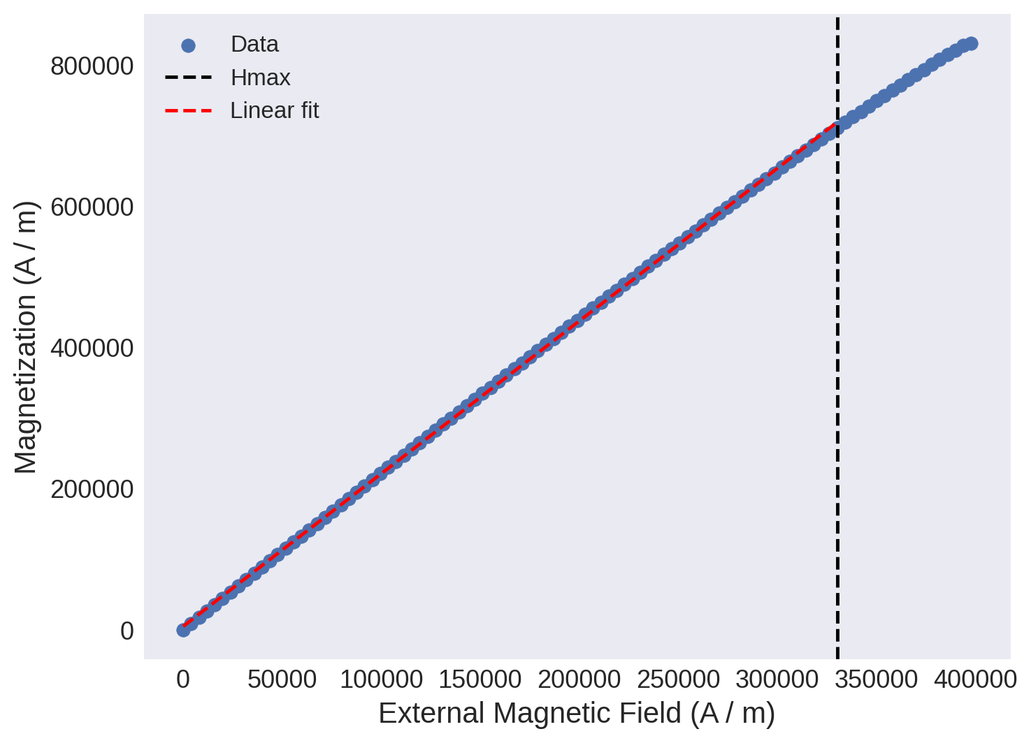
Linear segment#
Use mammos-analysis to find the properties of the linearized hysteresis loop.
results_linear = mammos_analysis.hysteresis.find_linear_segment(H_y, M_y, margin=0.05 * Ms.q.to("A/m"), min_points=5)
results_linear.plot();
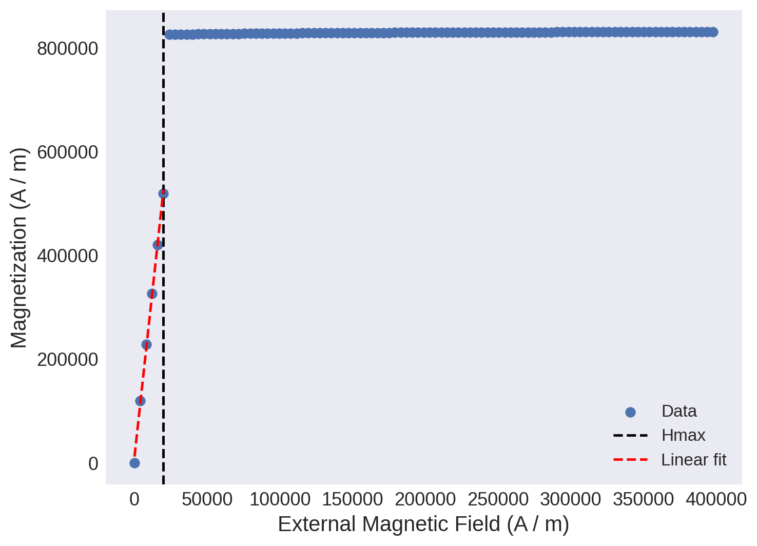
results_linear.Hmax # maximum field value of the linear region
results_linear.Mr # crossing of linear fit and y axis
results_linear.gradient # slope of the linear fit
Optimization#
Here we use Bayesian optimization to maximize Hmax by optimizing the lengths of the diagnonals \(s_x\) and \(s_y\) of the diamond.
from bayes_opt import BayesianOptimization
Define the objective function:
def objective(sx, sy):
    system.m = df.Field(
        mesh, nvdim=3, value=(1, 0, 0), norm=lambda p: in_diamond(p, sx, sy), valid="norm"
    )  # Change shape
    hd.drive(system, Hsteps=[[Hmin, tuple(Hmax.value), n]], verbose=0)  # Field sweep
    H_y = me.H(system.table.data["By_hysteresis"].values * u.Unit(system.table.units["By_hysteresis"]).to(u.A / u.m))
    M_y = system.table.data["my"].values * Ms.q
    results_linear = mammos_analysis.hysteresis.find_linear_segment(
        H_y, M_y, margin=0.05 * Ms.q.to("A/m"), min_points=2
    )
    return results_linear.Hmax.value
objective(19e-9, 39e-9)
3978.8735729668742
Running the simulation changes the system so we can view the new shape using:
system.m.sel("z").mpl()
We define the bounds over which the optimizer can search:
pbounds = {"sx": (3e-9, np.sqrt(2) * 50e-9), "sy": (3e-9, np.sqrt(2) * 50e-9)}
Initialize the optimizer:
optimizer = BayesianOptimization(
    f=objective,
    pbounds=pbounds,
    verbose=2,
    random_state=1,
)
We maximize the objective function:
optimizer.maximize(
    init_points=10,
    n_iter=20,
)
|   iter    |  target   |    sx     |    sy     |
-------------------------------------------------
| 1 | 3978.8735 | 3.123e-08 | 5.177e-08 |
| 2 | 3978.8735 | 3.007e-09 | 2.347e-08 |
| 3 | 51725.356 | 1.293e-08 | 9.252e-09 |
| 4 | 3978.8735 | 1.561e-08 | 2.639e-08 |
| 5 | 3978.8735 | 2.986e-08 | 3.948e-08 |
| 6 | 3978.8735 | 3.138e-08 | 4.939e-08 |
| 7 | 3978.8735 | 1.684e-08 | 6.245e-08 |
| 8 | 3978.8735 | 4.854e-09 | 4.839e-08 |
| 9 | 3978.8735 | 3.125e-08 | 4.082e-08 |
| 10 | 3978.8735 | 1.250e-08 | 1.641e-08 |
| 11 | 397887.35 | 6.905e-08 | 3.392e-09 |
| 12 | 397887.35 | 7.056e-08 | 3.088e-09 |
| 13 | 397887.35 | 7.003e-08 | 3.109e-09 |
| 14 | 397887.35 | 7.034e-08 | 3.032e-09 |
| 15 | 397887.35 | 7.058e-08 | 3.149e-09 |
| 16 | 354119.74 | 7.069e-08 | 4.440e-09 |
| 17 | 397887.35 | 7.027e-08 | 3.431e-09 |
| 18 | 397887.35 | 7.001e-08 | 3.102e-09 |
| 19 | 397887.35 | 7.046e-08 | 3.235e-09 |
| 20 | 397887.35 | 7.061e-08 | 3.444e-09 |
| 21 | 385950.73 | 7.051e-08 | 3.823e-09 |
| 22 | 397887.35 | 7.038e-08 | 3.029e-09 |
| 23 | 397887.35 | 7.046e-08 | 3.191e-09 |
| 24 | 397887.35 | 7.022e-08 | 3.127e-09 |
| 25 | 397887.35 | 7.039e-08 | 3.581e-09 |
| 26 | 397887.35 | 7.068e-08 | 3.212e-09 |
| 27 | 397887.35 | 7.024e-08 | 3.689e-09 |
| 28 | 374014.11 | 7.024e-08 | 4.054e-09 |
| 29 | 397887.35 | 7.046e-08 | 3.157e-09 |
| 30        | 385950.73 | 7.024e-08 | 3.829e-09 |
=================================================
print(optimizer.max)
{'target': 397887.35729668743, 'params': {'sx': 6.90545433922068e-08, 'sy': 3.392467321959973e-09}}
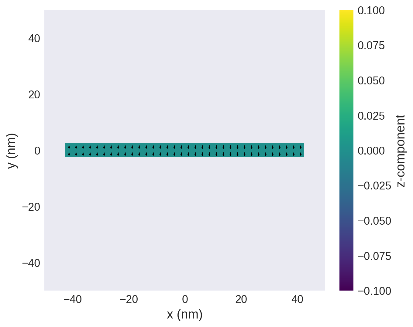
Lets run the simulation again with the best values to check the simulation and the shape.
sx, sy = optimizer.max["params"]["sx"], optimizer.max["params"]["sy"]
system.m = df.Field(mesh, nvdim=3, value=(1, 0, 0), norm=lambda p: in_diamond(p, sx, sy), valid="norm")  # Change shape
hd.drive(system, Hsteps=[[Hmin, tuple(Hmax.value), n]], verbose=0)  # Field sweep
H_y = me.H(system.table.data["By_hysteresis"].values * u.Unit(system.table.units["By_hysteresis"]).to(u.A / u.m))
M_y = system.table.data["my"].values * Ms.q.to("A/m")
results_linear = mammos_analysis.hysteresis.find_linear_segment(H_y, M_y, margin=0.01 * Ms.q.to("A/m"), min_points=2)
system.m.sel("z").mpl()
results_linear.plot();
We can also use the built in tools of ubermag to visualize the magnetization as a function of applied field directly.
data = md.Data(system.name)

drive = data[-1]

drive.hv(kdims=["x", "y"])
MODA for the workflow#
